Ken Dye
Mapping with only a bumper
Bumper Cart Mapping
The goal of this project was to build and program a robot capable of mapping and localizing itself in a 2-dimensional maze using only simple Ĺbumpĺ or touch sensors; no cameras, laser range finders, or sonars.
There are a couple of reasons why this is an interesting problem. First, robots with simple parts can be made smaller than those with more complex mechanics, allowing them to go into areas other robots might not fit. A nanobot that navigates by bumping into things would be more feasible than one that tried navigate based on input from a camera, for example.
Second, since a simple robot is also a (relatively) cheap and possibly small robot, this raises the possibility of coordinating the actions of many robots in a Ĺswarmĺ to achieve a goal. Combining the measurements of multiple robots mapping the same area would yield a more accurate map.
Third, the resolution of touch sensing is theoretically much better than range finders and doesnĺt require light to operate. These considerations give bump mapping a wider, or at least different, range of application than other methods.
Part 1: Building the Robot
The robot was built with a few main things in mind. The smaller the bumper is, or more precisely, the smaller the profile that the bumper projects onto the walls it collides with, the more accurately it can map them. A collision with a narrow bumper gives more exact information about where the object the robot collided with is. At the same time, the bumper needs to be wide enough to cover the entire profile of the robot so that the bumper is the only thing ever colliding with the walls.
The robot also needed a way to keep track of its movements. The simplest way to do this is to attach rotation sensors to the axles. At least two separate sensors would be needed, since the relative motion of the wheels needs to be known to control turning.
In the spirit of finding the absolute minimum capabilities required of a touch mapping robot, the robot was built with Legos. Legos have bump sensors and low-resolution rotation sensors. The size of the pieces do not allow for extremely accurate control or measurement (link to previous project.) Legos are, however, easy to assemble and program; many different ideas could be quickly implemented and tested.
In order to keep the robot small, only designs without a separate steering mechanism were used, allowing the robot to drive with only two powered wheels plus either caster wheels or skids. Steering was realized by turning the two wheels in opposite directions.
Driving and steering with two independently powered wheels, instead of a rack-and-pinion system, caused difficulties in getting the robot to drive in a straight line. Since Lego motors are not terribly well matched, providing each with the same power does not guarantee theyĺll each provide the same speed and torque; the robot will follow an arc instead of a straight line. Initially the robot was programmed with a PID tracking control to keep the rotation sensors for the left and right wheels matched to one another, but since with unmatched motors there is no steady-state for driving in a straight line, the robot moved as shown below.
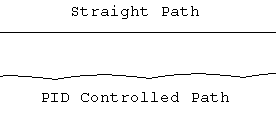
The path shown for PID controlled driving is longer than the straight path, but still covers the same distance. In the PID controlled case, then, the rotation sensors wonĺt be giving accurate measures of distance.
The other option for driving a two wheeled robot straightly is to use a differential gearing system. Driving straight is accomplished by powering the motor attached to the differential gear and turning is accomplished by powering the motor attached to one of the wheel axles. Unfortunately, to accommodate all this gearing the robot had to be made very large, and all the friction associated with gearing two wheels, two motors, and two rotation sensors, each geared at specific ratios, to a single drive train approached the limit of what a single motor Lego motor could handle (only one would be powered at any one time.)
The other main feature of the robot is the bumper. The mechanism for transferring a force applied anywhere on a 3 inch wide bumper to a small lego bump sensor needed to be very smooth and sensitive. It would be no good if, for example, the bumper had to be pushed hard because the wheels would likely slip at every collision and cause the measurements the robot made to accumulate error. The chosen design mounts the bumper on a relatively large hinge that is suspended over the bump sensor. Small rubber tires on ends of the bumper provide traction with the wall, allowing it to trip at even very small angles of incidence.
(pictures of cart)
The final robot design is shown in pictures above. It uses two separately powered wheels for driving, but without the PID control. The rotation sensors are geared to the drive axles with 12:1 reduction. This translates into a .0675 inches/tick resolution between the wheels and the rotation sensors. The next section describes how the robot collects and interprets map information, including how the problem posed by its non-linear paths was solved.
Part 2: Robot Control and Data Collection
To gather mapping data the robot was programmed to drive in a straight(ish) line until it hits something, record how far it went, back up, turn in a random direction, and drive off again. Letting this run long enough should, theoretically, collect enough points to make a map.
Since the robot doesnĺt drive in a straight line, it was programmed to log data from both the left and right wheel rotation sensors. Combining the readings from the two sensors makes it possible to determine the exact geometry of the path the cart followed.
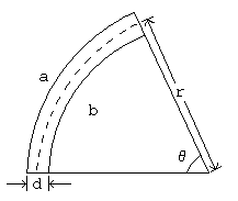
The diagram above depicts the robotĺs path. The wheelbase of the robot is d, a and b are the two rotation sensor readings. Determining r and theta allows the actual movements of the robot to be determined.
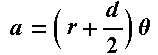
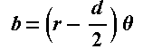
Solving the equations above for r and theta yields the following two expressions:
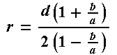
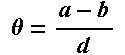
Thus for each a and b set a change in position and change in heading can be determined. These equations work equally well for the case that a or b is negative, meaning the robot was spinning in place.
In order to increase accuracy, the robot was programmed to log left and right rotation sensors readings for each stage of its movements: driving, backing up, and turning. This allowed the slight position change caused by the robotĺs inability to quite turn in place to be accounted for.
The control program was written in Not-quite-C. It is basically just a simple loop for driving, backing up, turning, and logging movement. It uses the Lego Mindstorms built in datalogging feature that allows for the storage of 16 bit integers that can be downloaded from the RCX unit through the IR port. Conveniently, the rotation sensor readings are 16 bit integer.
Given a set of sensor readings and the equations above, it is easy to plot the map points that the robot bumped. Vectors from each set of sensor readings can be determined and then rotated appropriately and added end to end. This was done in Matlab using the code linked here:
plotbumps.m
parsedatalogmore.m
curvdpath.m
getbumperpoints.m
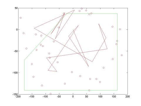
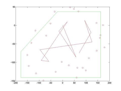
The picture above shows the results of adding end-to-end each movement. The green outline is roughly the space that the robot was confined to. The red path is the center of the robot and the red circles are in sets of three and correspond to the left, right, and middle of the robot's bumper. At least one in every set of three should fall on the green outline. However, after about the second hit, they do not. The only parameter to this model is the wheelbase. Because the wheels of the robot have a thickness, determining the wheelbase very precisely was difficult. The results pictured above are from the best estimate of that value.
Clearly there is too much error in the sensors to make a decent map from the raw data, and the final position that it gives for the robot is completely wrong. The next two sections describe how the raw data was processed to localize the robot within a known map and (hopefully) to make a map of an unknown area.
Part 3: Localization
The standard algorithm for localizing robots using noisy sensor data is the Monte Carlo method, detailed in this paper here. The algorithm works by basically seeding the map with possible locations and assigning them weights based on how likely a given sensor reading is to have come from that particle's location. This method works very well for sonars and rangefinders, and is relatively easy to implement. Making this work for a robot with only a bumper is somewhat harder.
One problem is that a measurement can only be made in one direction, and to take a measurement the robot has to move. Assigning a probability to a particle location is hard because it's difficult to get a good measure of the probability associated with a location; there is uncertainty in both the heading and the forward and lateral distance that the robot travels and the position after a movement is a function of both. This means that a particle could have ended up in a certain location from many other locations, and even in multiple ways from the same location. Each of those ways would have a different probability.
So, instead of trying to assign probabilities, a slightly different algorithm was implemented that uses the fact that the possible locations in the configuration space where a bump could occur is small. This 'bump-space' is a band inside the perimeter where the robot is facing outward. The algorithm works by basically seeding the map with particles, moving them by the logged robot movements with some added normally distributed error, and then removing the particles that are outside of the bump-space. The remaining particles are weighted evenly (by making enough duplicates of each one to equal the number of particles that were removed) and then the process is repeated. The algorithm was implemented in Matlab with the following functions.
localize.m
closetosegment.m
getsmear.m
onperimeter.m
pointinside.m
pointsinside.m
What follows is a sample run of the algorithm.
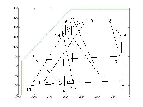
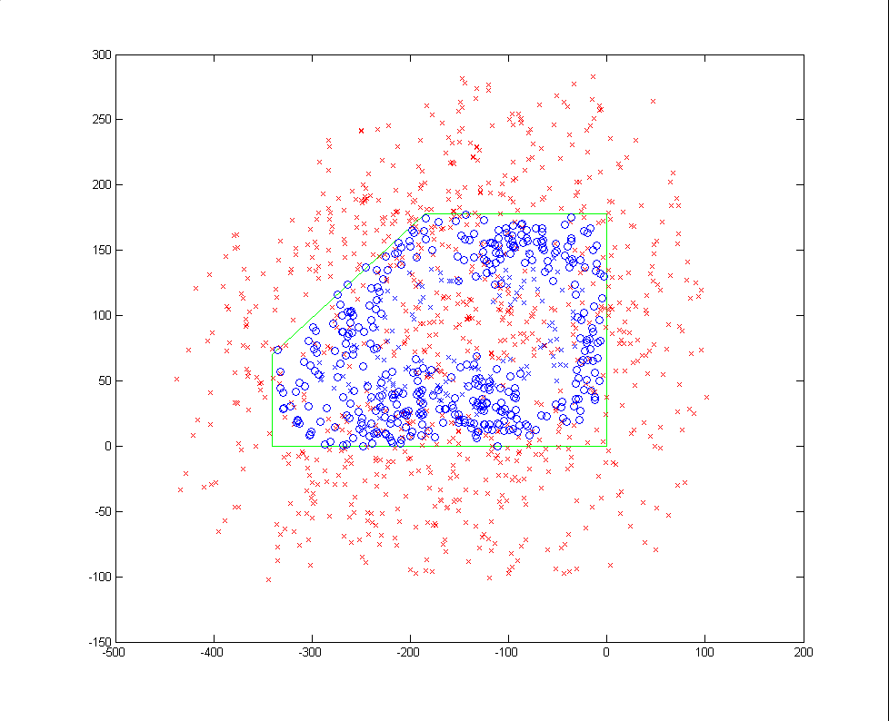
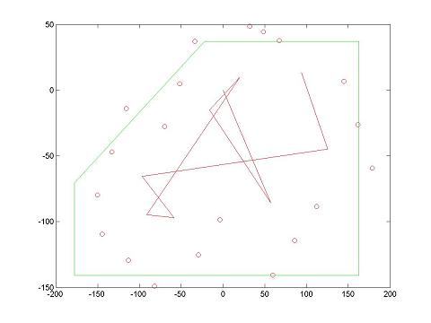
The first picture above is the actual path the robot took in this sample data run. It was created by drawing the path of the robot by hand as it ran. The second picture is the output of the localization algorithm after one iteration. It serves as a graphical illustration of the bumpspace. The red xs are robot locations that are outside of the bumpspace (they will be thrown out). The blue xs are robot locations inside the bumpspace, and the blue circles are points on the bumpers of configurations that are inside the bump space. The picture shows that the bumpspace is just inside the perimeter of the map, with the bumper facing out.

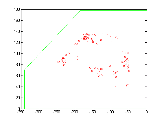
The left and the right pictures above are the results after the second and third iterations, respectively. The red xs are possible valid locations; invalid locations are not pictured. The increase in coherence in just this step is striking. The results are even more drastic for maps that are much more irregular.

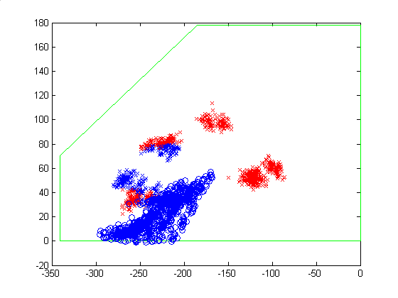
Pictured above are the bumpspaces after the fourth and fifth iterations. Again, the red xs are invalid locations, the blue xs are possible locations, and the blue circles points on the bumpers. By the fifth hit, the algorithm has nearly converged on the location and orientation of the robot.

Here are the results after eight hits: the left picture is the localization and the right picture is the raw data plotted end to end. The actual location of the hit was in the upper right corner with the cart facing north. The density of the cluster in the left plot is highest at the top, and this is pretty close to where the center of the cart was when its bumper hit the north wall. One can see from the right plot that the raw readings are starting to give a pretty skewed location. Taking this data I saw there was a fair amount of wheel slippage at hit 6 because the bumper hit the wall at an angle only slightly off of 90 degrees and flattened against it, destroying that small angle.
This is one of the challenges that the localization algorithm has to deal with. The errors between bumps tend to be either very small or very large, so it is difficult to find a way of distrubuting the particles that will work for both situations.

Pictured here are the results after 10 hits. The localizer does very well. The tenth hit did in fact happen with the cart in the southeast corner facing southeast. The two smaller clusters arrose after just two complete iterations from the relative tight cluster at hit 8 because of the large uncertainties that have to be given in the movement of the particles. This map, a rectangle with a corner cut off, looks pretty close to symmetric within the error spread used to move the particles, so clusters like this start small and have the potential to grow very large. When this happens it usually takes 3 or 4 more iterations for the location to reconverge.
The biggest difficulty in making this work was figuring out the right combination of parameters for the algorithm. It is very sensitive to the length of the wheelbase, the uncertainty in heading, the uncertainty in forward and lateral movement, the size of the bumper, and the size of the bump space (defined by the tolerance given to the pointinside function). Changing these uncertainties and tolerances has a large effect on how symmetric an area looks to the algorithm. The map used in the prior examples is not symmetric, but if one looks at it with sufficiently blurred vision, it looks symmetric. If the uncertainties and tolerances are too high, a more or less coalesced patch of particles will diverge into two quite easily from one move to the next.
Also, since the configuration space is three dimensional it needs a relatively large number of particles to cover it well. Results were only good for 700 or more particles. Less than that and some runs of the algorithm would not converge at all, meaning a movement resulted in no particles in the bump-space because there weren't any particles close enough to the robots actual position at that stage. This is only a problem, though, in that it makes the algorithm computationally intensive.
Conclusion
Even with the very noisy and inaccurate Lego sensors, and Monte Carlo-type localization algorithm works very well for a bump sensing robot. The main difficulties lie in finding the correct parameters for the algorithm that will make the bump space large enough to account for the error in the uncertainty in the lego sensors, but small enough that some asymmetry is preserved in the map so that successive iterations of the localization algorithm do not diverge.
The work on localizing was quite successful. In the future, it would be interesting to find a way of automatically zeroing in on the correct parameters for a localization model, perhaps by using a camera to separately observe the robot's movements and then correlate them with the robot's readings.
Links
All of the Matlab and NQC source code in a single zip file.
All of the diagrams used in this report in a single zip file.
Bibliography
Monte Carlo Localization for Mobile Robots by F. Dellaert, D. Fox, W. Burgard, and S. Thrun.