More about the FFT
Windowing
We used the specgram function that is built into Matlab to
produce spectrograms of the data. Specgram takes small segments
of a time sample, applies a window to each segment, and then takes the
FFT of that. The previous section mentioned how the FFT assumes
that the given sample repeats. The end of the original sample,
and the beginning of the first repetition are unlikely to line up
very well; in fact, there will most likely be a discontinuity on the
boundry. The
discontinuity causes problems because the FFT, wanting to model
the repeated signal exactly, adds a lot of high frequencies to
replicate the sharp drop from the end of the original sample
to the beginning of the first repetition. However, the
discontinuity is not really present in the original signal, so the
FFT provides an inaccurate representation of what's really going on.
In order to minimize this discontinuity, the time samples were
multiplied by a window. The Hanning window, which we used,
looks a lot like a Gaussian (bell curve). This window minimizes
the discontinuity because the start and end of the window are
very close to zero, forcing the end of one sample and the
beginning of the next to line up.
Are Short Time FFTs Reasonable?
We need to assure that using an FFT over a short
time gives us a reasonable approximation of the note. To do this,
we looked at the FFT taken over the entire note, and compared
it to the FFT taken over just a short time.
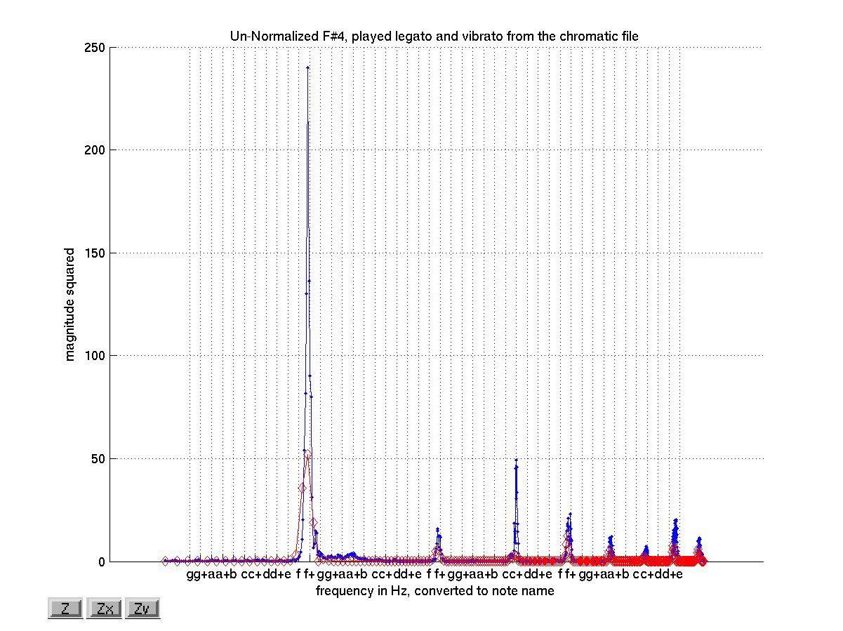
The above is the FFT of an F#4 played legato with vibrato.
The blue line is the FFT taken over the entire note (about
half a second), and
the red line is an FFT done with 4096 samples from the middle
of the note. Since our sampling frequency is 44.1 kHz, this
means the red line is the FFT taken over 0.093 sec. However,
it's hard to compare the two different lines because one
(the longer/blue) has many more data points than the other.
So what do we do? We normalize.
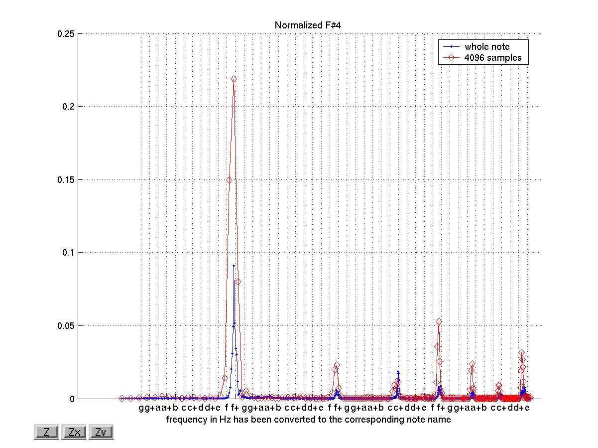
Above is the first normalization we tried,
which was normalizing the sum total
of each to one. This looks a little funny, because in almost
all parts, the red line is higher than the blue line. Even
in the sections where both are very small, the red line is still
higher than the blue line. The reason this FFT looks so odd is
that the long time sample has almost 5 times as
many data points as the short time sample.
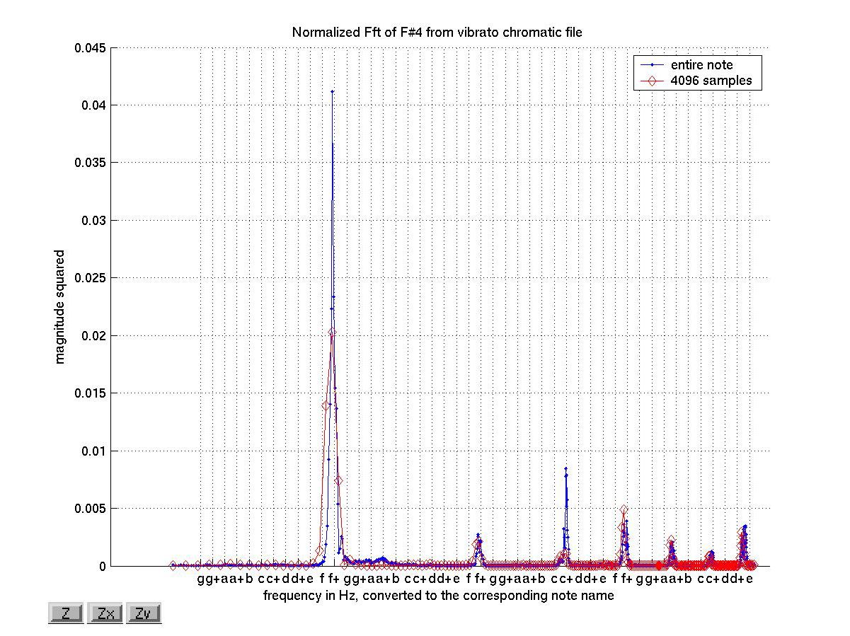
The normalization shown above normalizes the area under each curve to
one. This normalization is done by dividing each magnitude by
the sum of all the magnitudes times the frequency resolution.
Conclusions
In order to draw meaningful conclusions from the data, we must use the
proper normalization. The method that makes the most sense
in our case is the second normalization, because it accounts
for the fact that the long and short time samples have a different
number of data points. Overall, the patterns of harmonics look
similar for both long and short time samples. From this observation,
we conclude that it is reasonable to use short time FFTs with our
specified parameters
for violin pitch detection.
BACK
NEXT