Self-organizing Maps
Self-organizing Maps
Kevin Pang
Neural Networks
Fall 2003
Proposal
For my term project I will research and implement a Self-organizing Map (SOM).
I will submit an introductory guide to SOMs with a brief critique on its
strengths and weaknesses. In addition, I will write a program that implements
and demonstrates the SOM algorithm in action. This program will be for tutorial
purposes and will simply show how a SOM maps 3-dimensional input down to a
2-dimensional grid where geometric relationships between points indicate
similarity.
Back to top
Introduction
A Self-organizing Map is a data visualization technique developed by Professor
Teuvo Kohonen in the early 1980's. SOMs map multidimensional data onto lower
dimensional subspaces where geometric relationships between points indicate
their similarity. The reduction in dimensionality that SOMs provide allows
people to visualize and interpret what would otherwise be, for all intents and
purposes, indecipherable data. SOMs generate subspaces with an unsupervised
learning neural network trained with a competitive learning algorithm. Neuron
weights are adjusted based on their proximity to "winning" neurons (i.e.
neurons that most closely resemble a sample input). Training over several
iterations of input data sets results in similar neurons grouping together and
vice versa. The components of the input data and details on the neural network
itself are described in the "Basics" section. The process of training the
neural network itself is presented in the "Algorithm" section. Optimizations
used in training are discussed in the "Optimizations" section.
SOMs have been applied to several problems. The simple yet powerful algorithm
has been able to reduce incredibly complex problems down to easily interpreted
data mappings. The main drawback of the SOM is that it requires neuron weights
be necessary and sufficient to cluster inputs. When an SOM is provided too
little information or too much extraneous information in the weights, the
groupings found in the map may not be entirely accurate or informative. This
shortcoming, along with some other problems with SOMs are addressed in the
"Conclusions" section.
The rest of this site is dedicated to interesting applications of SOMS that I
have found. These range from powering search engines and speech pattern
recognition software to analyzing world poverty. A short description of these
projects and how they incorporated SOMs in them can be found in the
"Applications" section.
Lastly, I have coded an OpenGL program designed to demonstrate an SOM for
tutorial purposes. The executable, source code, and documentation on what the
program does and how to use it can be found in the "Demonstration" section.
The sources I used for this final project are listed in the "References"
section.
Back to top
Basics
Input Data
For the sake of clarity, I will describe how an SOM works by using a simple
example. Imagine a SOM that is trying to map three dimensional data down to a
two dimensional grid. In this example the three dimensions will represent red,
blue, and green (RGB) values for a particular color. An input data set for this
problem could look something like this:
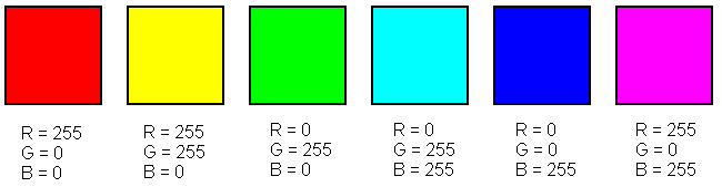
For this data set, a good mapping would group the red, green, and blue colors
far away from one another and place the intermediate colors between their base
colors (e.g. yellow close to red and green, teal close to green and blue, etc).
Neural Network
The neural network itself is a grid of neurons. Each neuron contains a weight
vector representing its RGB values and a geometric location in the grid. These
weight vectors will be used to determine the "winning" neuron for each input
and are updated based on its location during the training process. An
initialized neural network for this problem could look something like this:
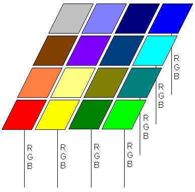
The squares in this picture represent the neurons and the descending verticle
lines show their intialized RGB values. Neuron weights can either be randomly
initialized or generated beforehand. In most cases random initialization is
sufficient as the SOM will inevitably converge to a final mapping. However,
pregenerating neuron weights can drastically improve convergence time and will
be discussed in the "Optimizations" section.
That covers the basics of a SOM. The input is a set of multi-dimensional
vectors and the neural network is a grid of neurons that each contain a weight
vector of the same dimensionality as the input vector. Now to explain the
algorithm used to train the neural network.
Back to top
Algorithm
The SOM learning algorithm is relatively straightforward. It consists of
initializing the weights as mentioned above, iterating over the input data,
finding the "winning" neuron for each input, and adjusting weights based on the
location of that "winning" neuron. A pseudocode implementation is provided
below:
Initialize weights
For 0 to X number of training epochs
Select a sample from the input data set
Find the "winning" neuron for the sample input
Adjust the weights of nearby neurons
End for loop
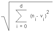
Finding the "Winning" Neuron
The algorithm used to find the "winning" neuron is a Euclidean distance
calculation. That is, the "winning" neuron n of dimension d for
sample input v (also of dimension d) would be the one which
minimized the equation:
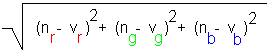
So for the three dimensional RGB example the "winning" neuron would be the one
which minimized:
Finding / Adjusting Neighbors
Adjusting the weights of nearby neurons can be done in several ways. The
algorithm for doing so involves first determining which neurons to scale then
how much to scale them by. The neurons close to the "winning" neuron are called
its "neighbors". Determining a neuron's "neighbors" can be achieved with
concentric squares, hexagons, and other polygonal shapes as well as Gaussian
functions, Mexican Hat functions, etc. Generally, the neighborhood function is
designed to have a global maxima at the "winning" neuron and decrease as it
gets further away from it. This makes it so that neurons close to the "winning"
neuron get scaled towards the sample input the most while neurons far away get
scaled the least (or in some cases in the mexican hat function, scaled away
from the sample input), which creates groupings of similar neurons in the final
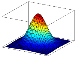
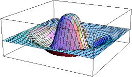
map. Below is an image of a three dimensional Gaussian function and a Mexican
Hat function:
The neighborhood function's radius is often decremented over time so that the
amount of "neighbors" decreases as training progresses. This is done to help
neurons initially adjust their weights to roughly where they want to be then
allow them to converge without being dramatically influenced by "winning"
neurons that are far away.
The amount to adjust each "neighbor" by is determined by the following formula:
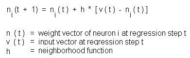
Similar to the neighborhood function, the amount to adjust each "neighbor" by
can also be adjusted over time so that initial neuron weight adjustment is
drastic but is less easily influenced as training progresses. This is done for
the same reasons mentioned for adjusting the neighborhood function's radius.
That covers the SOM algorithm for training its neural network. Neurons converge
to final weight values through a competitive learning scheme that adjusts them
to resemble nearby "winning" neurons. This process generates groups of similar
neurons in the final map
Back to top
Optimizations
Professor Teuvo Kohonen, along with a group of researchers at the Neural
Networks Research Center in Helsinki University of Technology, developed a few
optimization techniques for SOM training. Their project, WEBSOM, was designed
to organize massive document collections in real time using a SOM. In order to
accomplish this the research group had to develop methods for speeding up SOM
training time. The optimizaitons they came up with are detailed in their report
and involve reducing the dimensionality of input data, initializing neuron
weights closer to their final state, and restricting the search for "winning"
neurons. It is important to note that these optimization techniques were
designed specifically for their project and do not guarantee the same
clustering accuracy when used in other problems. However, the improvement in
training time does carry across all non-trivial SOMs.
Reducing Dimensionality
To provide some background information into the inspiration for reducing input
data dimensionality, I should mention that the initial input data for the
WEBSOM project was about 43,000-dimensional; each dimension corresponded to the
frequency of occurence of a particular word in a document. Furthermoer, the
original WEBSOM neural network contained over 1,000,000 neurons. Because of the
neural network's large size and the large dimensionality of the weight vectors,
training was a long and computationally heavy task.
Fortunately, the WEBSOM researchers came up with a way to reduce the
dimensionality of their data. They were able to do this by utilizing the Random
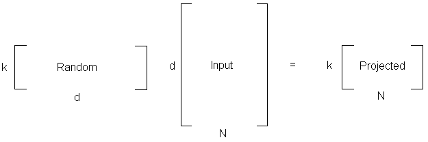
Projection algorithm. Random Projection takes d-dimensional data X
and projects it to a k-dimensional subspace (where k << d)
by mulitplying a random k x d matrix R, whose columns are
normally distributed vectors of unit length, with the input data X. This
produces a projected matrix of dimension k:
The reason Random Projection works is explained in the Johnson-Lindenstrauss
lemma:
"If points in a vector space are projected onto a randomly selected subspace of
suitably high dimension, then the distances between the points are
approximately preserved."
The "distance" between two points refers to the dot product of two
column vectors. Basically the Johnson-Lindenstrauss lemma says the similarity
between a pair of projected vectors will be the same, on average, as the
similarity of the corresponding pair of original vectors. In addition, the
WEBSOM researchers argued that if the original similarities between the points
were already suspect then there would be little reason to preserve their
relationships entirely. This justification allowed them to drastically cut down
the dimensionality of the input data and neuron weight vectors (from 43,000 to
500) without a noticeably drop in accuracy (from 60.6% to 59.1%).
Pregenerated Neuron Weights
Another technique the WEBSOM researchers utilized was a method of initializing
neuron weight values closer to their final state. This was accomplished by
estimating larger maps based on the asymptotic convergence values of a smaller
map. The researchers argued that constructing a smaller neural network,
training it with the input data, then interpolating/extrapolating data from the
smaller, converged map would generate a blueprint for the construction of the
larger map. This allowed the map to start its training closer to the converged
state which sped up the training process.
Restricting the Search for "Winning" Neurons
The last optimization technique mentioned in the WEBSOM paper was a method of
restricting the search for "winning" neurons as training progressed. Initially,
the search for the "winning" neuron must be thorough in order to find the best
fit neuron in the map. However, the WEBSOM researchers argued that once the map
starts to become smoothly ordered, the algorithm should be able to start
restricting the search for "winning" neurons to neurons close to the old
"winner". The researchers felt that after a significant amount of training, the
clusters would develop to the point where the location of "winning" neurons
would not move around much.
The gradual restriction of the "winning" neuron search turned out to be
significantly faster than performing exhaustive searches over the entire map
for every input. To ensure matches were a global best, a full search was
performed intermittently.
Back to top
Conclusions
Advantages
The main advantage of using a SOM is that the data is easily interpretted and
understood. The reduction of dimensionality and grid clustering makes it easy
to observe similarities in the data. SOMs factor in all the data in the input
to generate these clusters and can be altered such that certain pieces of data
have more/less of an effect on where an input is placed.
SOMs are capable of handling several types of classification problems while
providing a useful, interactive, and intelligable summary of the data. For
example, a SOM could be used in place of a Bayesian spam filter. Using a weight
vector similar to the one used in the WEBSOM project, a SOM should be able to
map e-mails onto a grid with clusters representing spam and not spam. Training
would be occur whenever the user marked an e-mail as spam or not spam. The user
would be presented with a graphical map of e-mail clusters, allowing him/her to
graphically view where an e-mail fell compared to other e-mails they had
previously marked as spam / not spam.
Finally, as the WEBSOM project showed, SOMs are fully capable of clustering
large, complex data sets. With a few optimization techniques, a SOM can be
trained in a short amount of time. Furthermore, the algorithm is simple enough
to make the training process easy to understand and alter as needed.
Disadvantages
The major disadvantage of a SOM, which was briefly mentioned in the
introduction, is that it requires necessary and sufficient data in order to
develop meaningful clusters. The weight vectors must be based on data that can
successfully group and distinguish inputs. Lack of data or extraneous data in
the weight vectors will add randomness to the groupings. Finding the correct
data involves determining which factors are relevant and can be a difficult or
even impossible task in several problems. The ability to determine a good data
set is a deciding factor factor in determining whether to use a SOM or not.
Another problem with SOMs is that it is often difficult to obtain a perfect
mapping where groupings are unique within the map. Instead, anomalies in the
map often generate where two similar groupings appear in different areas on the
same map. Clusters will often get divided into smaller clusters, creating
several areas of similar neurons. This can be prevented by initializing the map
well, but that is not an option if the state of the final map is not obvious.
Finally, SOMs require that nearby data points behave similarly. Parity-like
problems such as the XOR gate do not have this property and would not converge
to a stable mapping in a SOM.
Back to top
Applications
Here are links a few applications of SOMs I found along with a picture of their
SOM and a brief summary of their project:
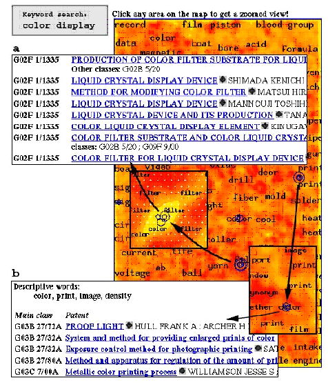
WEBSOM is a SOM that organizes massive document collections. It was developed
by Professor Teuvo Kohonen at the Neural Networks Research Center in Helsinki
University of Technology in the late 1990's. The project successfully created a
SOM that acted as a graphical search engine, classifying over 7,000,000 patent
abstracts based on the frequency of occurence of a set of words.
My Powerpoint presentation on Self-organizing maps and WEBSOM is available
here.
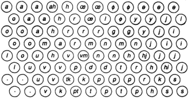
The Phonetic Typewriter is a SOM that breaks recorded speech down to phonemes.
It was developed also by Professor Teuvo Kohonen but in the late 1980's. The
documentation on the project can be found
here but requires the user to purchase it in order to view it. My
understanding of the article is therefore restricted to the information
presented in our lecture slides which state that the Phonetic Typewriter was
successful at translating speech into phoneme text in Finnish and Japanese. The
developers claim that 92% accuracy was achieved within 10 minutes of training.
The picture above is the SOM, which they called a phonetic map with the neurons
and the phonemes which they learned to respond to.
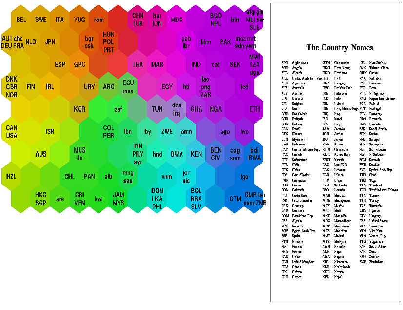
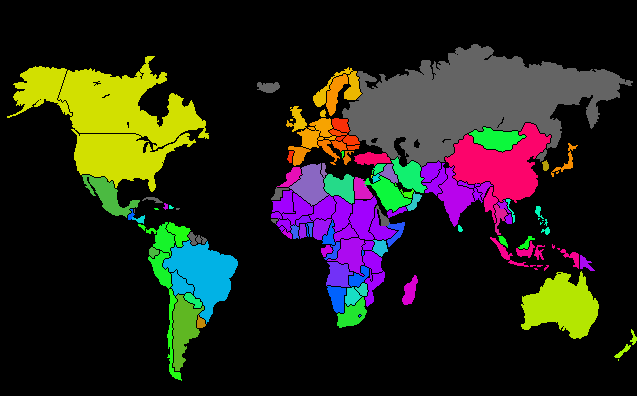
The World Poverty Classifier is a SOM that maps countries based on 39
"quality-of-life factors" including health, nutrition, education, etc. The two
pictures above show the SOM itself along with a key of country acronyms and a
map of the world where the countries have been colored in by their
corresponding locations in the SOM.
Back to top
Demonstration
Download
My OpenGL program demonstrating the SOM training algorithm is available
here.
Note: The program requires the glut32.dll file which is available
here. Place it in the c:\WINDOWS\system32 directory. The glut.dll file
is available here if you need it as well.
The sourcecode is available here.
Results
The program behaved very well after minor adjustments to constants in the
Gaussian neighborhood function. I obtained a wide spectrum of results depending
on my input set and how quickly I decreased the Guassian neighborhood
function's influence and radius. The program demonstrates an SOM training on a
randomly initialized grid of neurons. It is effective at forming distinct
clusters of similar neurons but sometimes has trouble developing the blended
transitions between these clusters.
Using the Program
The program runs on windows machines that support OpenGL and GLUT. It presents
the user with a randomly initialized map. Training can be toggled on and off by
pressing the 't' key. A console updates the user on whether training is
on or off as well as what training epoch the program is on. The map can also be
reset by pressing the 'r' key. In preliminary test runs the map
converged within 30 seconds to 1 minute.
Implementation Details
The map is a 100 x 100 grid of neurons each containing a weight vector
corresponding to its RGB value. The neuron weights are randomly initialized
using the computer's clock time as a seed. Training involves randomly selecting
an input from one of 48 unique colors, finding a "winning" neuron using
Euclidean distance, and adjusting the "neighborhood" weights. I used a Gaussian
function whose amplitude and radius decrease as the number of epochs increases
to determine how much to adjust the "neighborhood" weights. Because the neuron
weights are randomly initialized, the map converges differently each time.
Sometimes the map converges quickly and elegantly while othertimes the map has
difficulty in reaching stable equilibrium or filling in the gaps between
clusters.
Screenshots
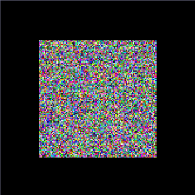
Randomly initialized map
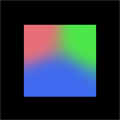
Map trained on shades of red, green, and blue
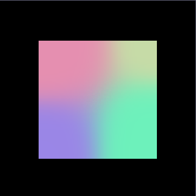
Map trained on shades of red, green, and blue with some yellow, teal, and pink
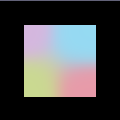
Map trained on shades of red, green, and blue with more shades of yellow, teal,
and pink
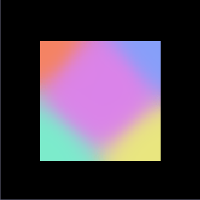
Another map trained on many shades of colors
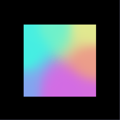
A well converged map with several clusters trained on 48 distinct colors
Back to top
References
| 1. |
Germano, Tom. Self-Organizing Maps.
http://davis.wpi.edu/~matt/courses/soms/ |
| 2. |
Honkela, Timo. Description of Kohonen's Self-Organizing Map.
http://www.mlab.uiah.fi/~timo/som/thesis-som.html |
| 3. |
Keller, Bob. Self-Organizing Maps.
http://www.cs.hmc.edu/courses/2003/fall/cs152/slides/som.pdf |
| 4. |
Kohonen, Teuvu et al. Self Organization of a Massive Document Collection.
Helsinki University of Technology, 2000 |
| 5. |
Unknown author. SOM Toolbox for Matlab.
http://www.cis.hut.fi/projects/somtoolbox/ |
| 6. |
Zheng, Gaolin. Self-Organizing Map (SOM) and Support Vector Machine (SVM).
http://www.msci.memphis.edu/~giri/compbio/f00/GZheng.htm |
Links
Here are the links posted on this website in case you missed them:
WEBSOM project
My powerpoint presentation on SOMs and WEBSOM
Slides from
class on SOMs
Phonetic
typewriter report
Classifying
World Poverty project
My SOM program
The sourcecode for my SOM program
My powerpoint presentation on this final project
Back to top