aka, Fourier analysis without the pain ...
Images are usually thought of as sums of individual pixels, weighted by the intensity (or 3 intensities, for 3 images) of those pixels. This part of the assignment asks you to investigate an alternative representation of images, that is as sums of frequency components, each of which is the size of the entire image. This part of the assignment asks you to build some tools that will help investigate the connection between the frequency and spatial representations of an image.
In general, the Fourier transform of an image has complex coefficients. With real images, the imaginary parts of these complex frequency coefficients always cancel out. The goal of this first problem is to demonstrate exactly how they cancel out.
Load the grayscale image sf.tif from /cs/cs153/Images/a2/fourier/sf.tif into your matlab workspace as A with
A = imread('/cs/cs153/Images/a2/fourier/sf.tif','tif');
Use the fftShow.m script (in the same place as imframe,
/cs/cs153/matlab/visioncode) to show both the image and its
frequency representation.
At this point, in your matlab workspace, B is the 256x256 matrix of frequency coefficients that is equivalent to the spatial image A. Because B is a matrix, its rows and columns run from 1 to 256, but it contains the uniform frequency (u=0, v=0) at its center, that is, at (129,129). (The fftshift function in matlab does this. If you look at fftShow.m, you'll see that this was done before the script ended.) What are the values of the B matrix of frequency coefficients for the nine frequency combinations with u = {-1,0,1} and v = {-1,0,1} ? (This is just a submatrix of B -- which submatrix is it?) Looking at these values (you can copy them directly to the html or link them in a file), why do the imaginary frequency components cancel?
Add the capability to "zero out" parts of the frequency representation -- that is, to set portions of the B matrix to zero. To do this, write a matlab function or script (or, perhaps, more than 1) that takes in some representation of the frequencies to be zeroed out, along with the fourier coefficients B and then returns a new coefficient matrix, suitably changed. In particular, make sure your function(s)/script(s) let you
To implement your filters, copy the fftShow script to a working directory and add the capability (now commented out) to change the fourier coefficients B and then redisplay the new spatial image (called D in the script). Also, add code to fftShow so that the newly abridged fourier coefficients appear too. (They should look like the old, except with a hole somewhere.) You can emulate code from earlier in the script to do this.
With these tools, generate spatial images and frequency representations of a 256x256 grayscale image of your choice (you can use the program xv to change the size of images easily). Feel free to use the San Fransisco image, if you'd prefer. Be sure to include
Try creating noise images (use the matlab rand function) and adding them to the grayscale image you investigated above. As we demonstrated in class, lowpass filters can smooth the resulting images.
Also, as you might guess, frequency representations are particularly good at removing
periodic noise (or unwanted information, at least) from images.
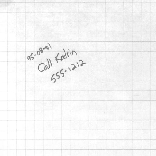
Use its frequency representation to remove the grid lines from
the following image. Don't download this one -- it's at
/cs/cs153/Images/a2/fourier/grid.tif. Notice that it's
512 x 512, which will require some adjustments, at least to the original
fftShow.m code.
Include in these results your "cleaned up" version of the above image, as wellas the results of adding noise and smoothing it with lowpass filters. What happens to an image as you let less and less of the high frequency components pass? (Give an example.)
Remember that you need to pursue only one extension in one part of the assignment, and it can be anything you'd like to investigate. These are only suggestions.