![]()
![]()
Reading: Russell and Norvig, chapter 4.
The search algorithms in the previous lecture treated all operators as having the same cost. For example, in route-finding, all paths of length 3 were considered equally good. In many applications, different operators have significantly different costs. For example, in route finding, some road segments are much longer than others. The search algorithm ought to take this into account.
Moreover, in certain problems, it is possible to estimate the distance from an intermediate state to the (nearest) goal state. For example, in route finding, we can estimate the distance to the goal location using the 2D straight-line distance. Such estimates can be used to guide search, often speeding it up significantly by preventing exploration of paths headed in the wrong direction.
Notice that the cost of a sequence of operators (e.g. a multi-step path) is the sum of the costs of the individual operators. In theory, this is not the only way to do things. But it is almost always used in practice.
Uniform-cost search requires that each operation have a cost associated with it. At each step in the search, the search algorithm selects the partial solution which has the lowest cost (from start to the current state) and extends it by one step (in all possible ways). This is implemented just like breadth-first search, except that the queue of partial solutions is kept in order of cost.
This algorithm behaves like breadth-first search except that it does "the Right Thing" when different steps cost significantly more than others. In route finding, the search tends to expand outwards at the same rate in all directions.
The textbook discusses something that they call "greedy search." It is a cut-down version of A* search (see below). This is an odd use of the term, which is usually used in a more general way in CS. I didn't find this special case particularly helpful in understanding and I can't think where this algorithm would be useful.
The idea behind A* (pronounced "A star") search is to pursue candidates in order of estimated cost from start to goal. The estimated cost is computed as follows:
f(state) = g(state) + h(state)
f is the estimated cost of the entire solution (when completed). g is the actual cost from the starting state to the current state. h is the estimated cost from the current state to the (nearest) goal state. These three function names are traditional. h stands for "heuristic" function.
A* is implemented by keeping a queue of partial solutions, sorted by f values. In the search loop, the algorithm removes the first partial solution from the queue. If it has reached a goal state, it returns the successful solution. Otherwise, it extends this solution by one step, in all possible ways. For each extension, it computes the estimate f and adds the extension to the queue in the appropriate place.
Route finding is a classic domain in which to apply A*. In this case, g is the actual distance along the roads. h is the straight-line distance between the end of the current partial route and the goal position. When applied to an actual map, A* finds the shortest path extremely well if the straight line distances are reasonable estimates of the actual road distance. If this is not the case (consider going from Lone Pine to Sequoia on the example map), it can end up searching paths that go in the wrong direction. However, on large maps, it rarely does worse than uniform-cost search.
Given "reasonable conditions" on the structure of the state/operation graph and the heuristic function h, A*
The main limitations of A* are that it is critically dependent on having a good heuristic function h, and it may a lot of memory to store the queue of partial solutions.
In order for A* to work properly, the following conditions must hold:
The first and second conditions involve search graphs of a type that you would probably never consider creating, unless you are a pure mathematician. The second condition exists to forbid paths in which the cost of steps decreases along the path, e.g. as the terms in a a geometrical series. A* can get stuck forever in such a path and fail to explore much better paths to the goal.
The third condition is the most likely to be violated in practice. It is required to prove the properties of A* listed above. However, many useful heuristics are not guaranteed to be underestimates. For example, straight-line distance could over-estimate the distance if the (x,y) coordinates of locations are rounded to finite precision.
Fortunately, A* "degrades gracefully" if the heuristic is not an underestimate. It will still return useful solutions. And these solutions will cost more than the optimal solution by an amount that is directly related to the extent to which h overestimates. Therefore, the A* algorithm is still useful even if h fails the third condition.
Suppose that the first item in the queue is a path p reaching the goal with cost k. Also in the queue is a path p' to node n, from which we can reach the goal via path s.
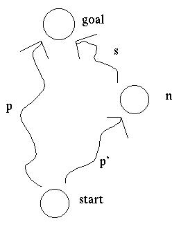
The actual cost of this second path s+p' is the actual cost of p' plus the actual cost of s. The actual cost of p' is g(n). The actual cost of s is >= h(n), because h always underestimates. So the actual cost of s+p' is >= g(n) + h(n) = f(n).
However, since the path p was before p' in the search queue, we know that the cost of p was <= f(n). Since p has reached the goal, its estimated cost is its actual cost. So the actual cost of p must be <= the actual cost of p'+s.
When implementing A*, it is important to always put a solution back into the queue, even if it has reached the goal. The first partial solution which reaches the goal is not guaranteed to be the shortest path. Rather, the solution must be allowed to percolate to the front of the queue: the shortest path is the first solution which is completed and reaches the front of the queue.
To understand why this is the case, suppose that we have a partial solution at the front of the queue which ends in state n and we extend this by one operation (with cost x) to reach the goal. Since our partial solution is at the front of the queue, all other partial solutions must have cost at least f(n) = g(n) + h(n). However, this is only an estimated cost. When we add the final extension, we learn the true cost g(n) + x. There may be other items in the queue with estimated cost between g(n) + h(n) and g(n) + x.
Suppose that a node can be reached by more than one path.
For some applications, we might want to put the node n in the search queue only once (along with the best path to n), so that we don't duplicate work exploring the paths leading onwards from n. However, in that case, what happens if we reach n later, via a shorter path? The above conditions on the heuristic function are not tight enough to prevent this from happening.
It is possible to handle this by setting up a system to remember all nodes that have been visited, and update their paths and evaluations if they are later revisited via a shorter path. Such an algorithm can be found in Nilsson, Nils J., Artificial Intelligence: A New Synthesis, Morgan Kaufman, 1998. However, the details are yucky.
A better solution is to add a condition to the heuristic function which ensures that, by the time a partial path reaches the front of the search queue, this path is the shortest path to its final node. This means that when we remove this partial path from the queue to extend it, we can put its final node on a "finished" list (or, more efficiently, in a hash table). If a path with that endpoint is generated later in the search, we can immediately discard it.
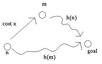
One way to state the required condition on h is "consistency." If it costs x to move from node n to node m, then h(n) <= h(m) + x. This condition is similar to the triangle inequality and, thus, satisfied by heuristics such 2D straight-line distance.
Another way to state the same condition is "monotonicity." That is, as we extend a path, its estimated total cost f never decreases.
To show that monotonicity and consistency are equivalent, suppose that we have a path from the start to a node n, and then a path from n to m with cost x, and finally a path from m to the goal. Then
     f(m) >= f(n) by monotonicity

     <==>   g(m) + h(m) >= g(n) + h(n)

     <==>   g(n) + x + h(m) >= g(n) + h(n)

     <==>   x + h(m) >= h(n) which is consistency
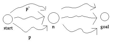
Now, let's show that monotonicity implies that a path reaching the front of the queue is the lowest-cost path to its final node. Suppose that the first item in the queue is a path p from the starting node to a node n. Suppose that there is another path p' in the queue which reaches a node m, and could be extended to a path p'+q which would reach node n.
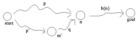
Because p is ahead of p' in the queue, f(p) is <= f(p'). Because f is monotonic, f(p'+q) >= f(p'). So f(p) <= f(p'+q).
Now, f(p) = g(p) + h(p) and f(p'+q) = g(p'+q) + h(p'+q). So f(p) <= f(p'+q) implies that g(p) + h(p) <= g(p'+q) + h(p'+q). But since p and p'+q both end at node m, and the h estimates are only based on the node (not the path to it), h(p) = h(p'+q). So g(p) <= g(p'+q).
A* can be applied in other domains. For example, we can evaluate states for the 8-puzzle (see Russell and Norvig for details) as follows:
These numbers are underestimates of the number of moves required to get from the current state to the goal state.
However, this example is unusual. For complex problems, it is frequently difficult to generate heuristic functions that are guaranteed to underestimate. Fortunately, as mentioned above, A* will still perform ok without this guarantee, as long as the heuristic function does not overestimate by too much.
A* search does wonderful things, but it can consume a lot of memory because it must store all open hypothesis on its queue. There are two ways to patch A* and reduce its memory consumption: (a) cross A* with iterative deepening or (b) use special memory-limited versions of A*.
Iterative-deepening A* (IDA*) is exactly what you'd expect from a hybrid of these two techniques. To implement it, you select a bound B on the estimated cost (f) of partial solutions. Then do DFS, halting whenever the estimated cost of a partial solution exceeds B. If no solution is found, increase B and repeat.
Well tuned, IDA* can perform like A* but with low memory usage. Badly tuned, it can perform extremely poorly. Achieving good performance requires an appropriate algorithm for increasing the bound B.
One option is to increase B to the smallest f value found among the states at which we halted the DFS. This works well if there are only finitely many values for f, so that the next iteration considers many more options than the previous one. However, it works incredibly poorly if each state has a different f value. Each iteration might then consider only one more partial solution than the previous iteration.
When f does have many different values, a better method is to increase f by a fixed constant E on each iteration. The constant would be chosen by considering the set of different costs for individual operations. This method guarantees a good running time. However, it may return a solution which costs E more than the optimal solution.
Simplified Memory-Bounded A* (SMA*) and Recursive Best-First Search (RBFS) are two algorithms for directly limiting the memory consumed by A*. The idea is to do A* but remove poorly-rated options from the queue if the queue gets too long. The challenge is then to ensure decent behavior if all the better-rated options fall through and we need to actually explore those poorly-rated ones.
To achieve this, these algorithms keep a record of all the partial solutions that have been considered, not just the maximally extended ones. Let's call a shorter solution an "ancestor" of solutions that have been made by extending it. Whenever a partial solution is to be deleted from the queue, its ancestors are updated so that they remember the best f value from any of their descendents that have been deleted. If the better-rated options fall through, these values allow the algorithm to make a rational choice of which low-rated ancestor nodes to re-explore.
The performance of SMA* and RBFS may be better or worse than A*. Apparently, it's hard to characterize when it will be better. The algorithms look complex: only worth examining in detail when you actually need to implement them.
This page is maintained by Margaret Fleck.