Computer Science 154
Problem Set 3, due Friday, March 9
Kinematics, Configuration Space, and Motion Planning

Name  __________________________

(This document is at http://www.cs.hmc.edu/courses/2001/spring/cs154/assignments/w3.html)

You may write the answers to these problems on the backs of these pages or submit them separately in hard copy or on the web. This problem set is due in class on March 8. Each lab group need hand in only one set of solutions, though all submissions will be graded.

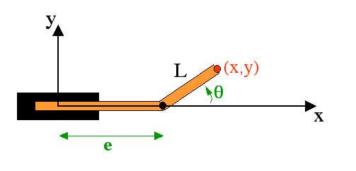
1. Manipulator Kinematics

Find the forward and inverse kinematic model for the PR manipulator depicted below. That is, for the forward kinematics find expressions for x and y in terms of the translational extent of the first link (e) and the rotation of the second with respect to the first (theta). For the inverse kinematics, find expressions for the robot's parameters (e and theta) in terms of x and y.

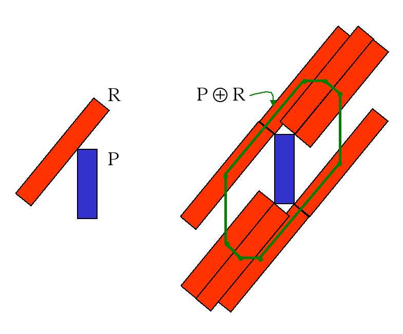
2. Minkowski Sums

The process of creating a configuration space for a mobile platform involved expanding, or dilating all of the obstacles by the shape of the robot. In class, for example, we looked at the resulting polygon (green) formed when a small blue obstacle is dilated by a larger red polygon representing a robot. (Admittedly, on these pages the colors will not be apparent.) Note that the choice of the centroid of R as an origin for the robot was arbitrary; we could choose any point.

This dilation operation is referred to as the Minkowski sum, which is often designated by .

Suppose A and B are two convex polygons, having a and b sides, respectively. In class, we noted that the maximum number of sides that AB could have is a + b. That is, the complexity of the resulting polygon is additive with respect to the original polygons.

Robots can generally be accurately modeled by convex polygons, but the same is not true of the obstacles in the world. It turns out that if A is convex and B is not convex, the Minkowski sum of the two can have O(ab) sides. As a result, the running times of motion planning algorithms that depend on the number of edges may be considerably higher than in the convex-obstacle case.

Question

Find a pair of polygons A and B that demonstrate that the Minkowski sum of a convex and nonconvex polygon can have multiplicative complexity. Note that this does not mean that the resulting polygon has exactly a * b sides, only that the resulting number of sides is proportional to that product. Be sure to indicate how to increase the number of sides of your A and B polygons such that the resulting Minkowski sum continues to have O(ab) sides.

3. Configuration Space and path planning

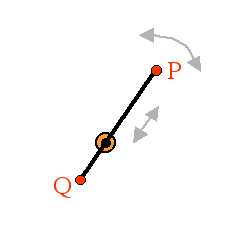
An HMC CS clinic, inspired by robot motion planning, has proposed a novel design for reading data from a hard disk. Each platter is read by two heads (P and Q), mounted on either side of a 10-millimeter-long armature. The armature passes through an axle at the center of the platter that both spins the arm and allows the arm to translate back and forth. The armature does not change size, but simply moves from one side to the other of the axle holding it.

The following diagram depicts this design. (The axle is perpendicular to the page.)

Another feature of this harddisk's design is that it will have a software controller that remembers bad sectors and makes sure that both of the read/write heads on the armature avoid them completely. (You might argue that this isn't a feature, I suppose...) In any case, the following diagram shows a number of bad sectors that the armature has to avoid on a particular platter.

In this picture, the obstacles are composed of circular arcs centered at the armature's axis and straight line segments extending radially from that center. The near arc of obstacle A is 2 mm from the center, obstacle B is 5 mm away, obstacle C's horns are 7 mm away, and obstacle's C's "indentation" is 9 mm from the center. Also, P and P* are both 8 mm from the center. (The armature is 10 mm long.)

Questions

1. Draw the configuration space for this mechanism, including the obstacles (the bad sectors) shown in the diagram above. Be sure to explain clearly what two parameters you are using to describe the configuration of the armature.



2. In a copy of this configuration space, draw a visibility graph and indicate a path within the visibility graph that would lead the read/write head labeled P from its current location to point P*. (This need not be the shortest path.)



3. In another copy of the configuration space, sketch an approximation of its voronoi diagram. Show a path that might be taken along it to get P to P*. (In order to get from endpoints P and P* to the voronoi diagram itself, choose some reasonable path.)



4. On the above "real" picture of the armature and obstacles (or a copy), roughly indicate point P's paths corresponding to the configuration space trajectories you created for the previous two questions.

4. Bug algorithms

Consider the two bug algorithms described in class. As a reminder, Bug 1 always circumnavigated obstacles; Bug 2 left an obstacle as soon as it reached the S-line at a point closer than the hit point.

In analyzing these algorithms we considered at worlds for which Bug1 traversed less distance than Bug 2 -- call these worlds "Bug 2 killers." We also looked at situations in which Bug2 traversed less distance than Bug1 -- call these worlds "Bug 1 killers."

Construct an algorithm that performs better than Bug 1 in the "Bug 1 killer" worlds and better than Bug 2 in the "Bug 2 killer" worlds. If you like, you may combine the two bug algorithms. Alternatively, you may start from scratch. Your algorithm should assume the same available information that the Bug algorithms assume (a known direction to the goal and known encoder readings). It does not have to outperform Bug 1 or Bug 2 for situations in which those strategies do well, but your algorithm should always reach the goal (as long as the goal is reachable). In addition to presenting an algorithm, briefly explain the tradeoffs you made in designing it.

5. Configuration space and an artistic challenge

Consider the configuration space (of the arm's endpoint) resulting when a circular obstacle of diameter 1 is centered 1.5 units from the arm's base. The goal of this problem is to develop a qualitative description of the configuration space, not a complete description of it. Thus, don't worry about the exact shape of the obstacle in C-space. Do, however, sketch at least three cross sections of it. If you're particularly ambitious, try drawing a 3d picture... .

If you would rather, feel free to use a tool like Mathematica or Matlab or Maple to render cross-sections of the configuration space and a full 3d picture of the obstacle, If you take this route, include any code you write.