The Mandelbrot set is a set of points in the complex plane that share an interesting property. Choose a complex number c . With this c in mind, start with
z0 = 0
and then repeatedly iterate as follows:
zn+1 = zn2 + c
The Mandelbrot set is the collection of all complex numbers c such that this process does not diverge to infinity as n gets large. There are other, equivalent definitions of the Mandelbrot set. If you took HMC's Math 11, for example, you may remember that the Mandelbrot set consists of those points in the complex plane for which the associated Julia set is connected. Of course, this requires defining Julia sets...
The Mandelbrot set is a fractal, meaning that its boundary is so complex that it can not be well-approximated by one-dimensional line segments, regardess of how closely one zooms in on it. In fact, the Mandelbrot set's boundary has a dimension of 2 (!), though the details of this are better left to the many available references.
Your first task is to write a function named inMSet(c, n)
that takes as input a complex number c and an integer
n. Your function will return a Boolean: True if the
complex number c is in the Mandelbrot set and False
otherwise.
In Python a complex number is represented in terms of its real part x and its imaginary part y. The mathematical notation would be x+yi, but in Python the imaginary unit is typed as 1.0j or 1j, so that
c = x + y*1jwould assign the variable c to the complex number with real part x and imaginary part y.
Unfortunately, x + yj does not work, because Python thinks you're using a variable named yj.
Also, the value 1 + j is not a complex number: Python assumes you mean a variable named j unless there is an int or a float directly in front of it. Use 1 + 1j instead.
Try it out Just to get familiar with complex numbers, at the Python prompt try
>>> c = 3 + 4jPython is happy to use the power operator (**) and other operators with complex numbers. However, note that you cannot compare complex numbers directly (they do not have an ordering defined on them since they are essentially points in a 2D space). So you cannot do something like
>>> c
(3+4j)
>>> abs(c)
5.0
>>> c**2
(-7+24j)
c > 2. However, you CAN compare the magnitude (i.e., the absolute value) of a complex number to the number 2.
To determine whether or not a number c is in the Mandelbrot set, you simply need to start with z0 = 0 + 0j and repeatedly iterate zn+1 = zn2 + c to see if this sequence of zs stays bounded, i.e., the magnitude of z does not go to infinity.
Of course, determining whether or not this sequence really goes off to infinity would take forever! To check this computationally, we will have to decide on two things:
The first value above (the number of times we are willing to run the z-updating process) is the second input, n, to the function inMSet(c, n). This is a value you will want to experiment with, but you might start with 25 as a reasonable initial value.
The second value above, one that represents infinity, can be surprisingly low! It has been shown that if the absolute value of the complex number z ever gets larger than 2 during its update process, then the sequence will definitely diverge to infinity. There is no equivalent rule that tells us that the sequence definitely will not diverge, but it is very likely it will stay bounded if abs(z) does not exceed 2 after a reasonable number of iterations, and n is that "reasonable" number.
So, to get started, write the function inMSet(c, n) that takes in a complex number c and a number of iterations n. It should output False if the
sequence zi+1 = zi2 + c ever yields a z whose magnitude is greater than 2 within n iterations. It returns True otherwise.
Check your inMSet function with these examples:
>>> n = 25
>>> c = 0 + 0j         # this one is in the set
>>> inMSet(c, n)
True

>>> c = 0.3 + -0.5j    # this one is also in the set
>>> inMSet(c, n)
True

>>> c = -0.7 + 0.3j    # this one is NOT in the set
>>> inMSet(c, n)
False

>>> c = -0.9+0.4j      # also not in the set
>>> inMSet(c, n)
False

>>> c = 0.42 + 0.2j
>>> inMSet(c, 25)      # this one seems to be in the set
True
>>> inMSet(c, 50)      # but on further investigation, maybe not...
False
Getting too many Trues? If so, you might be checking for abs(z) > 2 after the for loop finishes. There is a subtle reason this won't work. Many values get so large so fast that they overflow the capacity of Python's floating-point numbers. When they do, they cease to obey greater-than / less-than relationships, and so the test will fail. The solution is to check whether the magnitude of z ever gets bigger than 2 inside the for loop, in which case you should immediately return False. The return True, however needs to stay outside the loop!
As the last example illustrates, when numbers are close to the boundary of the Mandelbrot set, many additional iterations may be needed to determine whether they escape. We will not worry too much about this, however.
In order to start creating images with Python,
download the bmp.py file at this link
to the same directory where your hw7pr1.py
file is located. You will want to have the folder holding those files
open, because it is that folder (or Desktop) where the images will be
created.
Here is a function to get you started—try it out!
from bmp import *Save this function, and then run it by typing testImage(), with the parentheses, at the Python shell.
def testImage():
""" a function to demonstrate how
to create and save a bitmap image
"""
width = 200
height = 200
image = BitMap(width, height)
# create a loop in order to draw some pixels
for col in range(width):
if col % 10 == 0: print 'col is', col
for row in range(height):
if col % 10 == 0 and row % 10 == 0:
image.plotPoint(col, row)
# we have now looped through every image pixel
# next, we write it out to a file
image.saveFile("test.bmp")
If everything goes well, a few print statements will run, but nothing else will appear. However, if it worked, this function will have created an image in the same folder where bmp.py and hw8pr1.py are located. It will be called test.bmp and will be a bitmap-type image.
Both Windows and Mac computers have nice built-in facilities for looking at bitmap-type images. Simply double click on the icon of the test.bmp image, and you will see it. For the above function, it should be all white except for a regular, sparse point field, plotted wherever the row number and column number were both multiples of 10.
You can zoom in and out of bitmaps with the built-in buttons on Windows; on Macs, the commands are under the view menu.
Just for practice, you might try making larger images—or images with different patterns—by changing the testImage function appropriately.
Some notes on how the testImage function works...
There are three lines of the testImage function that warrant a closer look:
Ultimately, what we are trying to do is plot the Mandelbrot set on a
complex coordinate system. However, when we plot points on the
screen, we manipulate pixels. As the example above shows, pixel
values always start at (0, 0) (in the lower left) and grow to
(width-1, height-1) in the upper right. In the example above width
and height were both 200, giving us a reasonably sized image.
However, if we created a one-to-one mapping between pixel values and
points in the complex plane, our real value would be forced to range
from 0 to 199 and our imaginary value would be forced to be between
0 and 199. This is not a very interesting region to plot the
Mandelbrot set, because the vast majority of these points are not in
the set (so our image would be mostly empty).
What we would like to do is to be able to define any complex coordinate system we want, and then visualize the points in that coordinate system. To do this, we need to project the pixel values (i.e., the location were we will possibly put a dot on the screen) onto this coordinate frame (i.e., the _actual points in the complex plane_). In other words, given a pixel, to determine whether to put a dot there, you need to first figure out what point it corresponds to on the complex plane and then test to see whether that complex point is in the Mandelbrot set.
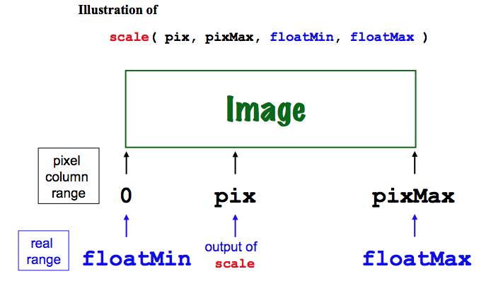
To help with this conversion back and forth from pixel to complex coordinates, write a function named scale(pix, pixNum, floatMin, floatMax) that takes in four things: pix, an integer representing a pixel column, pixNum, the total number of pixel columns available, floatMin, the floating-point lower endpoint of the image's real axis (x-axis), and floatMax, the floating-point upper endpoint of the image's real axis (x-axis).
The idea is that scale will return the floating-point value between floatMin and floatMax that corresponds to the position of
the pixel pix, which is somewhere between 0 and pixNum. This diagram illustrates the geometry of these values:
Once you have written your scale function, here are some test cases to try to be sure it is working:
>>> scale(100, 200, -2.0, 1.0)  # halfway from -2 to 1
-0.5

>>> scale(100, 200, -1.5, 1.5)  # halfway from -1.5 to 1.5
0.0

>>> scale(100, 300, -2.0, 1.0)  # 1/3 of the way from -2 to 1
-1.0

>>> scale(25, 300, -2.0, 1.0)
-1.75

>>> scale(299, 300, -2.0, 1.0)  # your exact value may differ slightly
0.99
Note Although we initially stated it as something to find x-coordinate floating-point values, your scale function works equally well for either the x- or the y- dimension. You won't need a separate function for the other axis!
This part asks you to put the pieces from the above sections together
into a fucntion named mset(width, height) that computes the set of
points in the Mandelbrot set on the complex plane and creates a bitmap
of them. For the moment, we will use images of width width
and height height, and we will limit the part of the plane to
the ranges:
-2.0 ≤ x or real coordinate ≤ +1.0
and
-1.0 ≤ y or imaginary coordinate ≤ +1.0
which is a 3.0 x 2.0 rectangle.
How to get started? Start by copying the code from
the testImage function—those pixel loops using
col and row will be the basis for your mset
function, as well.
There are at least five things that you will have to change:
The variable width and height inputs provide the opportunity to create both large images (if you're patient) and small images (for quicker prototyping to see if things are working). You might first try
>>> mset(300, 200)to be sure that the image you get is a black-and-white version of the many Mandelbrot set images on the web. Then, you might want to try a larger one...
mset function
As we've discussed previously, Magic Numbers are simply literal numeric values that you have typed into your code. They're called magic numbers because
if someone tries to read your code, the values and purpose of those
numbers seem to have been pulled out of a hat... For example, your
mset function may have called inMSet(c, 25) (at least mine did). A newcomer to your code (and this problem) would have
no idea what that 25 represented or why you chose that value.
To keep your code as flexible and expandable as possible, it's a good idea to avoid using these "magic numbers" for important quantities in various places in your functions. In fact, in this case, we'd rather not define any values directly in our code. Rather, we want the user of our function to be able to pass them in.
Modify your mset function so that it has the following signature (as described at the top of this page):
mset( width, numIterations=25, coordinateList=[-2.0, 1.0, -1.0, 1.0], outFile="mset.bmp")
The
parameters to this funciton are as follows:
height = width*(vertical range)/(horizontal range)This will ensure that the aspect ratio of the resulting image is valid.
Next, experiment with different values of numIterations. In particular, you might try the values
numIterations = 5in addition to our default value of 25.
numIterations = 10
and
numIterations = 50
Finally, play around with the coordinate list to "zoom in" on an interesting piece of hte Mandelbrot set's boundary.
Remember that if you like a particular image and don't want to overwrite it, you can simply change its name from test.bmp to something else.
The next two extensions are completely optional. You don't have to do them, but they are fun... and pretty!
You don't have to use black and white!
The image object representing a BitMap supports changes to the "pen color" through the method call
image.setPenColor(Color.GREEN)where the actual color can be any of BLACK, BLUE, BROWN, CYAN, DKBLUE, DKGREEN, DKRED, GRAY, GREEN, MAGENTA, PURPLE, RED, TEAL, WHITE, or YELLOW. By setting both the pixels out of the set as well as those in the set, you can create many variations in background and foreground...
Try it out!
Images of fractals often use color to represent how fast points are diverging toward infinity when they are
not contained in the fractal itself. For this problem, modify your
mset function so that it plots points that escape to infinity more quickly in different colors.
Thus, have your
mset function plot the Mandelbrot set as before. In addition, however, use at least three different
colors to show how quickly points outside the set are
diverging—this is their "escape velocity." Making this change
will require a change to
your inMSet helper function, as well. Perhaps copy, paste, and rename inMSet so that you
can change the new version without affecting the old one.
There are several ways to measure the "escape velocity" of a particular point. One is to look at the resulting magnitude after the iterative updates. Another is to count the number of iterations required before it "escapes" to a magnitude that is greater then 2. An advantage of the latter approach is that there are fewer different escape velocities to deal with.
Choose one of those approaches—or design
another of your own—to implement mset in color.
Note on defining your own colors
You are not limited to using the predefined colors listed above. You can create a color object, similar in spirit to the bitmap objects
that we have been working with, through the following code:
mycolor = Color(red,green,blue)where red, green, and blue are integers between 0 and 255 inclusive. They indicate how much of those color components the object mycolor will have. After this definition, mycolor may be used just like any of the predefined colors.
When you are done playing—it can be surprisingly
addicting!—you are done with lab. Be sure to submit your
hw7pr1.py file and your mset.bmp file... .