Natural Deduction - Introduction & Elimination Rules

“I could not help laughing at the ease with which he explained his process of deduction.”
—Sir Arthur Conan Doyle

Natural Deduction is a formal proof system that most closely corresponds to the kind of reasoning we normally see in mathematics. The rules (allowed proof steps) can be divided into three groups: Introduction Rules, Elimination Rules, and Classical Rules.

Introduction Rules

The introduction rules let us prove formulas involving logical operators in the most direct and obvious ways.

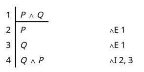
The $\land I$ rule (“and introduction” or “conjunction introduction”) lets us prove a brand-new conjunction in a way that reflects our intuitive understanding of the $\land$ operator: we can prove the formula ${\cal A}\land {\cal B}$ immediately once we have proved ${\cal A}$ and ${\cal B}$:

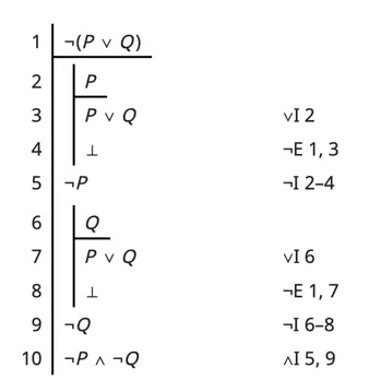
Similarly, the $\lor I$ rules (“or introduction” or “disjunction introduction”) lets us prove a brand-new disjunction in a way that reflects our intuitive understanding of the $\lor$ operator: we can prove the formula ${\cal A}\lor {\cal B}$ immediately once we have proved either ${\cal A}$ or ${\cal B}$:

(Although technically there are two rules, instead of calling them $\lor I_1$ and $\lor I_2$ we will just use the name $\lor I$ and you can infer from context which of the two rules we are referring to.)

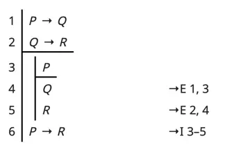
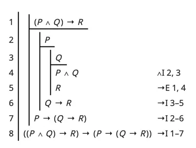
The $\to I$ rule (“arrow introduction” or “implication introduction”) if we can show the conclusion does indeed follow from the premise:

In this rule, the notation

means “a subproof that (temporarily) assumes ${\cal A}$, and manages to prove ${\cal B}$.” The horizontal line separates the assumption from the following derivations, and the vertical line indicates the scope of that assumption (how far into the proof we can rely on the temporary assumption ${\cal A}$.

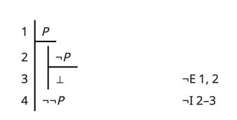
The $\lnot I$ rule (“not introduction” or “negation introduction”) lets us directly prove a negation (i.e., that the formula isn’t true), if we can show that assuming the formula is true would lead to a contradiction:

Finally, the $\bot I$ and $\top I$ rules let us prove $\bot$ and $\top$ directly. The only way to prove $\bot$ is to show we’ve already reached a contradiction. But proving $\top$ is trivial (and boring), because $\top$ is always true:

Elimination Rules

The elimination rules let us use existing formulas according to their logical connectives. For example $\land E$ lets us derive consequences from an existing conjunction, while $\to E$ lets us derive consequences from an existing implication.

What can we immediately conclude from a conjunction? That each of the individual conjuncts is true.

(As with $\lor I$, we use the same name for two closely related rules and context will tell us which one we are referring to.)

What can we immediately conclude from an implication? If the premise of that formula is also true, we can conclude the conclusion is true:

In fact, $\to E$ is the same rule as Modus Ponens from the Hilbert System, just under another name.

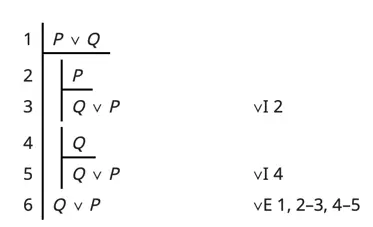
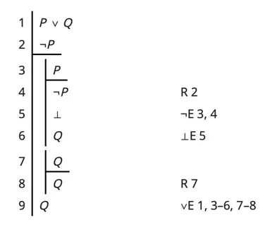
The $\lor E$ rule may look a bit complicated, but it is exactly the reasoning principle that mathematicians call “Proof by Cases”. If we already know the disjunction ${\cal A}\lor {\cal B}$ is true, and (by checking both cases) we discover that some conclusion ${\cal C}$ follows regardless of whether it is ${\cal A}$ or ${\cal B}$ that is true, then the conclusion ${\cal C}$ is definitely true:

Next, the most direct way we can draw a conclusion from an existing negation is if we discover that negation is part of a contradiction:

In fact, $\lnot E$ is the same rule as $\bot I$. The rule has two names, depending on whether we think of it as making use of an existing negation, or recording the existance of the contradiction.

Finally, there is the $\bot E$ rule. Since asserting $\bot$ is a way of announcing we’ve reached a contradiction, and since (according to our definition of entailment) any formula follows from a contradiction, we can derive any formula we want from $\bot$:

(There is no $\top E$ rule, because the fact that $\top$ is true gives us no information at all, so there’s no useful consequence we can derive from it.)

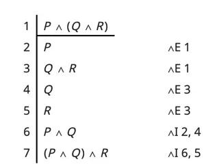
Example Proofs

$P\land Q \ \ \vdash \ \ Q\land P$

---

$P\land (Q\land R)\ \ \vdash\ \ (P\land Q)\land R$

---

$P\to Q,\ Q\to R\ \ \vdash\ \ P\to R$

---

$\vdash ((P\land Q)\to R) \to (P \to (Q\to R))$

---

$P\lor Q\ \ \vdash\ \ Q\lor P$

---

$P\lor Q,\ \lnot P\ \ \vdash\ \ Q$

---

$P \vdash \lnot\lnot P$

---

$\lnot(P\lor Q)\ \ \vdash\ \ \lnot P\land \lnot Q$