Recurrent Neural Networks
for Linear Programming

Brad Tennis

Linear Programming

Basic Theory

Linear programming seeks to minimize or maximize a linear function over a set of linear constraints on the function variables. In standard form, a problem may be expressed as:

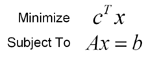
The column vector c contains the coefficients of our objective function, the constraint matrix A holds the coefficients of our constraint functions and the constraint vector b holds the constraint values. There is also the implicit constraint that all values in the solution vector x are nonnegative. For the rest of the paper, let us use n as the number of primal variables and m as the number of primal constraints.

Notice that we may convert a maximization to a minimization problem by negating the coefficient vector c. We may also convert inequality constraints into equality constraints by adding an additional variable known as a slack variable. For instance, suppose we had a constraint

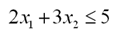
To convert this into an equality constraint, we add a new variable to remove the "slack" in the inequality.

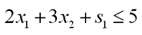
In the case that we have a greater than or equal to inequality, we simply add the negation of the slack into the constraint. As for any other variable, there is an implicit constraint that all the slack variables be nonnegative.

Based on a linear programming problem called the primal problem, we may construct a second problem known as the dual problem. We formulate the dual problem as:

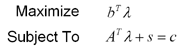
where A, b and c are taken from the primal problem. Notice that where the primal problem was a minimization problem, the dual problem is a maximization problem. Additionally, we have explicitly included the slack variables s, whereas in the primal problem they were folded in to the primal variables x. In the dual problem, we make the implicit constraint that all values in s are nonnegative, but values in the lambda vector may be anything.

Duality theory, as explained in Wright provides a useful result for our purposes. The value of the objective function at the dual problem is a lower bound on the solution to the primal problem, and the primal problem is an upper bound on the solution to the dual problem. That is:

Further, for linear programming problems, the function values are equal when the solution to both the primal and the dual problem are optimal.

This suggests the formulation of a new problem, called the primal-dual which combines the primal and dual of a linear programming problem into one problem. To create this problem, we must define an objective function, a set of constraints. The solutions to the primal dual problem are vectors whose first n entries correspond to x, whose next m entries correspond to the lambda vector and whose last n entries correspond to s. As our objective function we use:

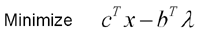
From the above result, the minimum of this function is 0 and it occurs when we have a solution to both the primal and the dual problem. However, as you will see, the choice of objective function is largely irrelevent.

For our constraints, we simply combined the primal and dual constraints into one set and add the addtional constraint that the value of the objective function be 0. This means that any feasible point of the primal dual problem contains an optimal solution to the primal and dual of our original problem.

For a primal-dual problem we also define a quantity known as the duality measure, whose formula is given by:

This value should go to zero as the iterates approach an optimal solution.

So, using the primal-dual problem, we have reduced our task from finding a minimum subject to constraints to merely finding a feasible solution.

The design for this network is based heavily on the deterministic annealing network proposed in Wang. In fact, the network architecture, shown in the image below, is the same.

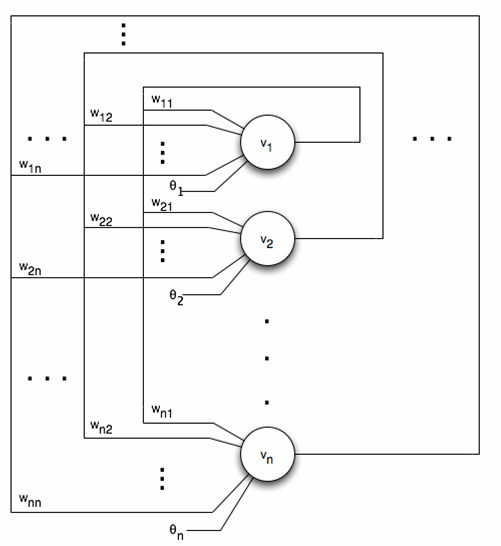
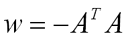
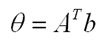
In this network, the weights matrix is defined to be

The network keeps track of two vectors, u(t) and v(t). The vector v(t) represents the output of the neurons at time t and the vector u(t) represents the input to the transfer function F(u(t)) at time t. The value of v at time 0 is randomly chosen from the hypercube bounded by 0 and vmax, where vmax is a program parameter representing the maximum value of an iterate. The value of u at time 0 is equal to v(0).

At each iteration, the step vector is calculated as:

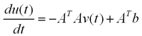
Notice that this is the net input to the neurons at the current time. We must now use this input to find the value of v. First, we update the u vector as follows.

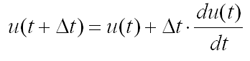
Essentially, the u vector is acting as an accumulator that keeps the sum of all the net inputs to the network over all time. Once we have calculated u, we must transform u into our neuron output v. For the components of u corresponding to x and s we use the following transfer function to keep iterates between 0 and vmax. The parameter xi affects the steepness of the sigmoidal transfer function.

For the values in u corresponding to the lambda vector, we use a linear transfer function as there are no explicit bounds on the values in the lambda vector

Lastly, we set the neuron output vector v to the value returned by the transfer function F(u), completing one iteration of the network.

First notice that the transfer function F(u) is monotonically increasing. Therefore, if we increase the vector u, we also increase the value of v. Let us now consider the step vector. We may rewrite its equation as

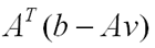
Let us consider the quantity in parantheses. This may be thought of as the error in our current iterate. If, for some constraint, the value of the error is negative, then Av is too large. So, we want to attempt to reduce the value of Av. To do so, we may need to either increase or decrease v depending on the sign of the values in the constraint matrix. Since F(u) is monotonically increasing, we may increase the value of v by increasing u and decrease v by decreasing u. Therefore, the step vector may be seen as taking a step towards a feasible point v*.

We also see that as iterates approach the feasible point v*, the length of the step vector must decrease to zero as the error also goes to zero. This allows the network to converge to a feasible value through repeated iteration of the above dynamic.

Results

Example Problem 1

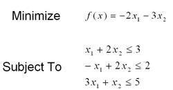
The first example problem is formulated as follows:

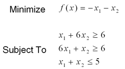
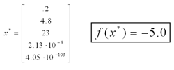
The problem was first converted into standard form by adding 3 slack variables. Using a timestep of .005, a vmax and a xi of 1, the network converged to the optimal solution in less than 1 million time steps. Below we see the values assigned to each of the 5 primal variables (including the slacks) at the end of 1 million iterations.

Below are some graphs detailing the progress of the network. On the left is the duality measure, mu, which should be zero at an optimal point. In the center is the magnitude of the error vector, which should go to zero for an optimal point. Lastly, on the right is the trajectory of the first two primal variables as they converge to an optimal solution. Click on the pictures to bring up a new window with a larger version.

Duality Measure

Error Magnitude

Primal Variable Trajectory

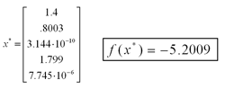
The second example problem is drawn from Wang. It is formulated as:

Again, we first convert to standard form by adding slack variables. We then convert the problem to its primal dual form and build a network as outlined above. Using the same parameters as above, the network converged to an optimal solution in less than 1 million time steps. Below are the outputs of the primal variable neurons upon completion. The optimal solution here is x=1.4 and y=.8, which differs slightly from the given solution. The network is set to terminate when the length of the error vector is sufficiently small, so it may terminate before an optimal solution is reached. Were the network to have continued running, it would have continued to converge to x=1.4, y=.8.

Below are some graphs detailing the progress of the network. On the left is the duality measure, mu, which should be zero at an optimal point. In the center is the magnitude of the error vector, which should go to zero for an optimal point. Lastly, on the right is the trajectory of the first two primal variables as they converge to an optimal solution. Click on the pictures to bring up a new window with a larger version.

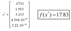
This problem is the second linear programming example drawn from Wang. It's objective function and constraints are:

This problem is already in standard form, so we need not add any additional variables. A network was cconstructed from this problem's primal-dual and operated under the default parameters given above. As before, the network converges in less than 1 million timesteps to the optimal solution given in Wang.

Below are some graphs detailing the progress of the network. On the left is the duality measure, mu, which should be zero at an optimal point. In the center is the magnitude of the error vector, which should go to zero for an optimal point.Click on the pictures to bring up a new window with a larger version.

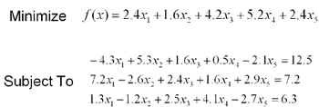
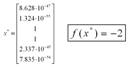
The specification of the final example problem is given by:

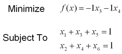
It's easy to see from inspection that the optimal solution is to set x3 and x4 equal to 1 and set everything else equal to zero. The problem is already in standard form, so we need not add any additional variables. When the network based on this problem is run with the default parameters, it converges to the optimal solution in less than 1 million timesteps.

Below are some graphs detailing the progress of the network. On the left is the duality measure, mu, which should be zero at an optimal point. In the center is the magnitude of the error vector, which should go to zero for an optimal point. Click on the pictures to bring up a new window with a larger version.

1. Wang, Jun. "A Deterministic Annealing Neural Network for Convex Programming." Neural Networks vol. 7 no. 4 (1994): 629-641. http://www2.acae.cuhk.edu.hk/~jwang/pdf-jnl/NN1994.pdf




2. Wright, Stephen J. Primal-Dual Interior-Point Methods. Philadelphia: Society for Industrial and Applied Mathematics, 1997.



3. Hagan, Martin T, Howard B. Demuth, and Mark H. Beale. Neural Network Design.