Monte-Carlo Localization: from Tragedy to Triumph!
Daniel Lowd
CS 154: Robotics
Spring 2003
Introduction
We live in uncertain times, times of war, times of economic hardship,
times of cultural change. In such a world, we must hold our
beliefs carefully, having the courage to apply them yet the grace to
evolve them. Belief without action yields nothing, but brittle
beliefs are easily broken. Robotics is much the same: machines
that interact with the world face uncertainties at every level. I
hope to address one of the most basic questions: where am I? For
the first few weeks, I will focus on resolving a robot's position in a
known and static environment. Through Monte-Carlo Localization
[1], a robot may combine the information of many readings in many
positions, narrowing its position down to the few most probable.
For the final weeks, I will attempt to build the map at the same
time, a process known as Simultaneous Localization And Mapping, or SLAM.
The methods of Monte-Carlo Localization may be combined with
expectation maximization (EM) to yield the most likely map and position,
given a set of locations and sensor readings.
None of these methods is new: all have been published and implemented
on multiple systems. I hope to explore some of the limitations of
these methods when implemented on the Nomad 200 in a simulator.
Through simulation, I can easily add random and systematic errors
in noise or positioning, then observe the effects on the algorithm.
My goals are first accuracy, then robustness, then flexibility.
A robot algorithm must first be effective before other factors are
worth considering. I consider reliability in the face of
uncertainty and errors to be an important secondary goal, given the
unpredictability of the real world. Flexibility in this case
represents making fewer assumptions so the algorithm is effective in
more environments with fewer modifications required.
Progress
Part 1: Map reading and particle filtering
I first attempted to implement MCL by working on the MCL assignment,
starting from Zach Dodds' code. Methods were included for reading
in a map file, computing the distance to the nearest wall in each
direction, updating particle locations, and moving the robot using the
keyboard. All of this proved to be quite helpful. After some
hacking, I managed to get a mostly working implementation. I
played around with parameters a bit and tried out a few maps to verify
that it seemed to work, but did not do extensive experimentation.
This system represented a step towards a viable implementation,
rather than the solution itself. It should be noted that I never
had much success localizing in the maze I developed. Part of this
is likely issues with my implementation that I need to address.
Part of it is also probably parameter tuning. I didn't spend
too much time on this, since I was eager to spend my time tuning the
final algorithm, with all features implemented.
This critical weakness of this first implementation was that it
required absolute knowledge of the robot's angle. If the robot
were equipped with a compass, this assumption could perhaps be made.
However, I wished to relax it, so my robot could localize itself
starting from any position or angle, with no special knowledge other
than its sonars and an accurate map. I also decided to support
maps with angled walls, not just vertical and horizontal ones.
This functionality seemed important in the real world, where not
everything is straight.
The major challenge of these two features turned out to be not robotics
so much as geometry. The problem to be solved could be summarized
as determining the point where a ray intersects a line segment, if the
two intersect at all. Given a location and angle for the robot, I
had to determine the distance to the nearest wall, each wall being
represented as a line segment, so I could compare this theoretical
distance with actual sonar readings. When the robot's sonars only
point in the cardinal directions, this is trivial. When the sonars
may be at arbitrary angles, this requires substantial angle
normalization, use of arctangent, and finally, the law of sines.
Debugging it turned out to be very difficult, so I wrote a
separate program to generate random test cases of a form that would be
easy to solve and compare my algorithm to the known answer. This
helped me uncover the final bug in the algorithm, as well as a number of
bugs in my testing code. All told, it took many hours to restore
the original functionality of my program with this new method.
Even when this was done, it was hard to use it with sonar because the
sonar was less accurate and less consistent. Even with no noise
added, the sonar disagreed with my calculations on the distance to a
wall. Part of this showed up as a systematic error -- the sonar
underestimated the distance by about 9-10 inches, though it varied.
I suspect that this is because my calculations work from the
center of the robot, while sonars are positioned on the outside, so the
result should be off by the radius of the robot. I tried
accounting for this in my computations, but there were so many other
errors that it was hard to tell how much effect it was really having on
the results. Another source of error could be how sonar works --
my calculations assume straight lines, while sonar goes out in a cone.
Still, this should not have affected the experiments I was
running, which used a perpendicular wall.
Another sonar-related issue was corners. Specifically, a sonar
may bounce off of a corner, resulting in the maximum reading rather than
the appropriate distance. This can cause all of the most accurate
position guesses to be discarded in favor of less accurate ones. I
attempted to remedy this by skipping past any sonars that read the
maximum reading, and only focusing on ones that provided more specific
distance information. Now, however, it seems to be having more
difficulty closing in on the right location.
I also found it necessary to mess with the number of particles and the
standard deviation used in the model a fair bit. The reason for
this seems to be that the standard deviation in the model must account
for not only the error in the sonar readings, but also the error in
particle placement. If the sonar reading is off by a distance of
10.0 units and the nearest particle is 10.0 units away from the correct
location, then the actual error may be as great as 20.0. If the
standard deviation of the error is assumed to be 10.0, then the result
is two standard deviations from the mean rather than one. This
gets still more complicated with a three-dimensional state space, as
it's harder to quantify the effect of being off by 10 degrees, and only
1/18th of the particles will randomly be within 10 degrees of the true
angle anyway.
In fact, that very reason may be part of why I had so little success
once I added robot angle as a third variable. The system tended to
converge to inaccurate areas or not converge at all during my limited
experiments. Experimentation was slower than I anticipated, since
the graphics routines are so inefficient. Generating a bitmap and
writing it to a file each time might be faster. 100 points is
manageable, but 5,000 or even 500 is noticeably slow. (Even though
drawing points rather than circles did provide a sufficient speed-up.)
Overall, I feel I've made a great deal of progress, but localization is
clearly not complete. Conceptually, it's done -- the algorithm is
fully implemented in the code. Practically, it doesn't perform
very well at all. Experimentation, debugging, tuning, and analysis
will hopefully suffice to improve it.
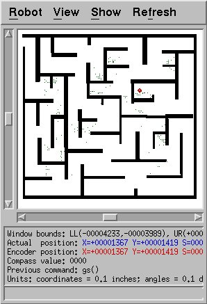
Part 2: Dual-MCL and a Hybrid Algorithm
Simultaneous localization and mapping seemed far too ambitious, when
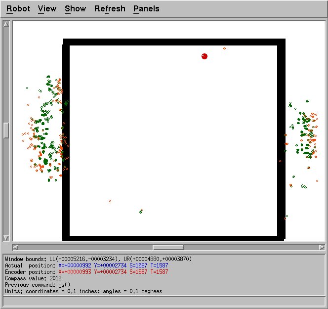
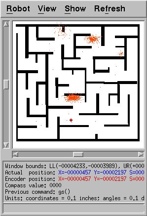
localization itself was broken. The figure below shows an extreme
example. It was possible to confuse the algorithm so that almost
all possible points were outside the room!
I decided to try out my code on the 2D localization problem, since I
had already solved that for a short homework assignment. What I
uncovered was the same systematic error mentioned before. By
taking into account the radius of the robot into account, I was able to
mostly fix this problem.
Once this modification (and perhaps a few other fixes) had been made, I
was able to successfully do 2D localization in a maze. Sometimes.
When the particles were placed right to begin with. What I
was really trying to accomplish was consistently successful 3D
localization.
To tackle this, I implemented a more complicated version of Monte-Carlo
localization: by adding particles sampled from the configuration space,
conditioned on the last sensor reading, one can theoretically achieve a
much more robust solution [2]. Unfortunately, the article I read
did not specify all the details. For example, how is one supposed
to sample particles from the configuration space? Furthermore, how
does one determine the probability that each came from one of the
particles from the last time step? Though several methods were
listed, none was clear enough for me to be sure of how it applied.
They made numerous references to kd-trees, so I took some time to
learn about kd-trees and how they worked.
My final conclusion was that I could sample particles based on sensor
readings by first uniformly generating particles, then computing their
theoretical sensor readings, and finally building a kd-tree keyed on the
16 different readings. The sampling process would then consist of
taking a set of sensor readings, adding noise, and finding the point
with the nearest readings, as cached in the kd-tree. By adding
different random noise each time, I could sample many of these at
random, and was not restricted to selecting only the k nearest
neighbors of the actual sensor reading. This seemed
probablistically justified.
The weighting process I used was to generate a guess of the newly
sampled particle's possible previous location and scale its likelihood
based on the density of the prior particles in that area. Since
density can be measured as points/unit volume, I was build a kd-tree of
the prior particles, keyed on location in three dimensions, and used the
size of the hyper-rectangles at the leaves as indications of the
relative density at various locations.
I successfully implemented all of this in several steps. First, I
developed my own kd-tree code. Though code is publicly available,
I needed something efficient, flexible, and with as little encapsulation
as possible. I wanted to be able to traverse the tree myself
rather than relying on some object method to give me the information.
I wrote a test program to help me debug it, and only continued
when I was satisfied that it worked.
Next, I wrote the code for building the uniformly-sampled sensor
readings kd-tree. This took additional debugging, because I
suddenly had to deal with duplicate values in my kd-trees. For a
while, there were issues with infinite recursion, since the kd-tree
building code couldn't split up the many points for which all sensor
readings are 255 inches. Eventually, I modified the tree structure
so that a leaf could contain many data points and finished debugging it.
The sampling code and weighting code were more straightforward, though
they had some bugs at first, especially the weighting code. When
finished, I was able to place the robot in various locations and see
what particles it generated. Some locations seemed to work better
than others.
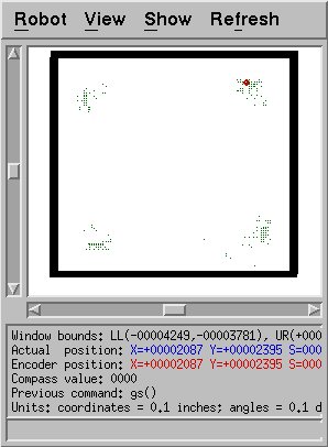
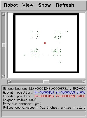
Here is an example of successful sampling: since the space is
rectangular, close to square, sensor readings that indicate a corner
could imply any of the four corners. The algorithm accurately
selects points from all corners.
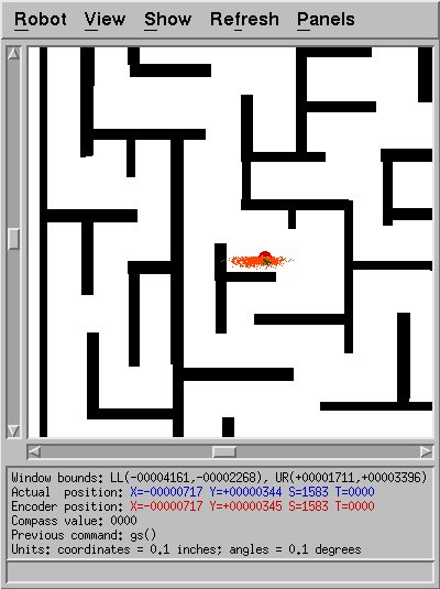
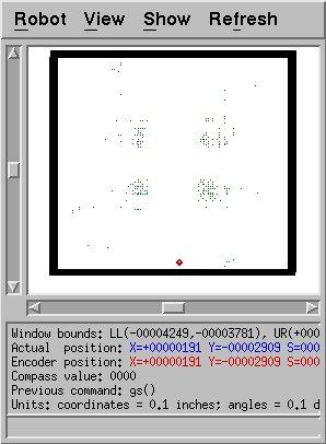
It seems to work fairly well in the maze as well. Since the maze
is complicated and has many similar-looking locations, the particles are
spread out a fair bit, but some of them are quite near the true
location of the robot. This is a good sign.
Another location in the maze furhter confirms this. Not only are
some particles near the robot's true location, there are particles in
many other dead-ends that look similar, as one would expect.
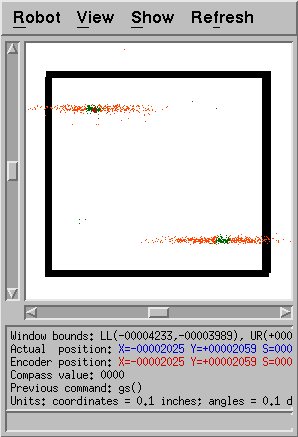
Unfortunately, this method has at least one serious weakness.
This figure shows the particles generated when all sensors had
their maximum readings, 255.0. One would expect more particles in
the middle near the actual location of the robot. Unfortunately,
it is very unlikely that a central point will ever be chosen.
There are 16 sensor readings and each receives noise representing
the sensor error and additional noise for each sampled particle.
Since the error added is Gaussian, there's a 50% chance that any
given sensor reading is changed so that it is less than 255.0. The
probability that all of them remain at 255.0 is thus 1/2^16 = 1/64,000.
While the added sampling noise could change some of those values
back to 255.0, it's likely to change just as many in the opposite
direction. Since the noisy sensor readings have values under
255.0, the sampled particles are likely to be less than 255.0 inches
from some wall, which is exactly what we see.
This shows the biggest weakness of my overall approach: maxed out
sensor values are not modeled accurately. With a real robot, if
the actual distance is 1,000, it would be highly unlikely for the sensor
to read 240.0 or 236.0. But supposing one assumes that actual
sensors are noisy the exact same way as simulated in my code.
Then in order to accurately model the probability density function
of the sensors' true values, one would need to include priors for each
distance. That is, since a true distance over 255.0 is much more
common than a true distance of 236.0, if the sensor value is 240.0
(after noise), then 255.0 may be its more likely original value than
236.0, even though 236.0 is closer. I thought a bit about ways to
correct this -- for example, use the uniformly sampled sensor readings
to construct a probability distribution to fix this -- but decided that
would be outside the scope of my project.
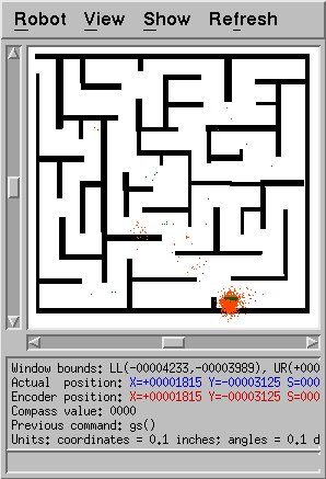
The second-biggest weakness of my approach also has to do with sensor
modeling. In the robot's displayed location, all of its sensor
readings are 255.0 except for one. Because it's so close to the
wall, one one sonar bounces back to the robot; the rest bounce away and
never return. Since only one of the 16 sensors is less than 255.0,
we have almost the same distribution as shown before, when the robot
was in the middle. My clearance computations would have predicted
much lower readings on diagonal sonars than actually occurs here;
therefore, more accurate points will rarely be chosen in such a
situation. Better sensor modeling would fix this problem. I
declared this problem outside of the scope as well, and hoped the
situation would be tolerable overall.
When I combined the two methods, I did so as suggested in the paper:
select some fraction of the particles by sampling given the sensor
readings; select the remainder by moving all previous particles are
reweighting, as in regular MCL. These methods together did seem to
yield a better solution than either alone. I tried several values
for the fraction before settling on 0.1, which seemed to be enough to
fix the problems with my original MCL solution.
This shows a successful localization on a simple map, using the more
robust method. Unfortunately, it took 32 steps to achieve this
solution. Due to the random placement of particles to begin with
or the noise added to the sensor readings, the algorithm quickly
selected one of the two likely positions shown and placed all of the
particles there. Due to the symmetry of this map, both solutions
should be equally likely, but due to chance, only one was selected.
The particles added by sampling did help give the other solution a
chance, but it remained the minority over many, many moves. The
reason for this is that once one solution had more particles, the
competing solution had to have more accurate particles in order to
change the distribution. However, the solution with more particles
was more likely to have at least some particles that were very
accurate. Over 32 steps, it did stabilize, and I believe it will
in general, but it can be slow.
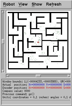
Trying this on the maze map worked, too, but also took a while.
This shows the early hypothesis of the algorithm: note that very
few points are near the true location of the robot. However, over
time this was eventually fixed, as shown in the figure belows.
Overall, this modified algorithm is clearly more robust than MCL,
even with poorly modeled sensors and improper probabilities.
References
[1] F. Dellaert, D. Fox, W. Burgard, and S. Thrun. Monte Carlo localization for mobile robots.
In Proceedings of the IEEE International Conference on Robotics and
Automation (ICRA), 1999.
[2] S. Thrun, D. Fox, W. Burgard, and F. Dellaert. Robust Monte Carlo Localization for Mobile
Robots. Artificial Intelligence, vol 128, 1-2, pp 99-141,
2001.
Appendices
Source code for Monte-Carlo localization, and various testing code: mcl.zip