Final Report 1Updated TimelinePLAY BOTBALL BY APRIL 30TH!Progress UpdatesBasic MotionBasic motion control has been set up for the robot. This includes basic functions for turning left and right by a specified angle (in degrees), for moving forward and backwards at a specified speed, and stopping. Due to asymmetries in the robot and motors, these motions aren't perfect. While it moves in a fairly straight line forwards and backwards, it may not stay straight for longer distances. Additionally, while the turning functions are pretty good, they probably do not have more than 5 degrees of resolution and accuracy. There were some physical changes made to the bot to help make this movement more accurate. There were some initial problems with turning related to the castor wheels. These would take a moment to turn and line up with the rotation of the robot, which would give variations in how far it turned, depending on whether or not the wheels were already aligned with the direction of motion. These were replaced with simple skids, which cause slight drag, but that error seems to be minimal. Additionally, there were some issues with moving in straight lines. The wheels were noticed to be rubbing against the sides of the robot, which we thought might be causing problems. The internal framework of the robot was restructured, and the motors were re-glued to LEGO pieces to minimize rubbing. The first attempt resulted in the axles being misaligned on the motors, so they had to be re-glued once more. However, now they are aligned correctly and no part of the wheels are rubbing against LEGOs. LocalizationWe currently have an idealistic odometry model running on the robot that estimates its x and y position based solely on the six holed odometer wheels on the outsides of the chassis. The model is similar to ones that we have covered in class while doing kinematics, as explained below.
In Figure 0 the gray rectangles indicate the robot's wheels and the blue line indicates their common axis. The model assumes that the wheels are mounted at the center of the robot, thus the robot's center starts out at the origin and moves with the center of the axis. The model also assumes no wheel slippage during maneuvering. To derive the formulas for the position and orientation of the robot
we want to first start by finding R and a in terms of
variables that we know the values of. So, we are given
l from measurements and we know dL and dR from
sensor readings, and this is sufficient to create a system of eqations
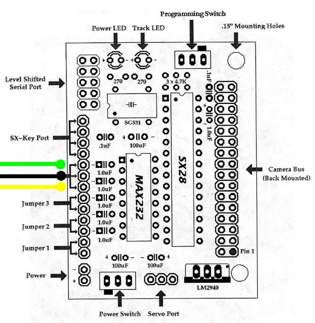
to solve R and a. The derivation then looks as follows: dR = (R - l/2)a R = dR/a + l/2 dL = ((dR/a + l/2) + l/2)a = dr + la Therefore a = (dL - dR)/l And so R = dR/a + l/2 = (ldR)/(dL - dR) + l/2 = = l(2dR + (dL - dR))/(dL - dR) = l(dR + dL)/(dL - dR) Therefore R = l(dR + dL)/(dL - dR) In practice the program currently calculates x,y and theta in the manner described above, after each movement made by the robot. The robot keeps track of its current position and orientation, and simply updates the values each time these calculations are made. The dL and dR values are derived from the differences in the number of changes in odometry since before the movement and the directions the motors turned during the movement. The next step, is to sparate these calculations into their own process that will run most likely between changes in motor direction, and incorporate information about the arena from our sensors to get a more accurate task specific localization scheme. In order to get the best localization possible, the ideal approach would be to integrate our odometry with visual, sonar, line-detection, and bump sensing to get the best possible idea of where the robot is located. Unfortunately, the techniques used in the literature such as Markov-models [6] or Monte Carlo Localization [7] are poorly suited to our task and robot. The simple Markov model works well for Dervish, but that is because it operates in a smaller configuration space (essentially one-dimensional along the network of corridors) and has sensor information that is easier to abstract. We initially considered dividing up the playing area into a grid of location cells, but the number of such locations becomes very large in order to approach any precision for our location, especially when the dimension of rotational pose is added. This causes problems both in requiring tuning of a very large number of transition probabilities as well as eventually becoming too complex to calculate using the HandyBoard. Also, the types of input used to trigger possible transitions between states are much less well defined. Due to the higher-dimensional continuous configuration space and variety of sensors, our robot would probably locate effectively using Monte Carlo methods; unfortunately, the HandyBoard doesn't have enough processing power for full-on MCL. Because of these limitations, we plan to base localization primarily on odometry data, using some sensor data to "sanity check" and compensate for wheel slippage and any encoder error or uncertainty. The localization will not be used for all tasks of the robot as most will be based on homing in on a particular visible goal such as a ball, toilet paper tube, or basket. Some degree of localization will be necessary, however, to identify which side of the board we are on, important because the scoring of objects in green baskets is based on which side the green basket is on at the time. CameraWe had trouble getting the camera to work consistently with the computer and the HandyBoard. Eric tracked the problem down to a loose connection between the CMUCam board and the telephone wire (CAT3 wire with RJ11 connection) which connects to the Handyboard and the computer. Eric and Adrian determined the correct wiring for connecting the CAT2/RJ11 wire to the TTL port on the CMUCam. A color coded diagram is here. Green is ground, Black is transmit, and Yellow is receive. Adrian re-soldered the connection, and now the camera works much more consistently with both the Handyboard and the computer.
To assess the ability of the CMUCam to locate and track the orange Poof Ball, we place an orange ball inside the nest against a white background and see if the CMUCam can locate the ball and accurately track it. The setup we used is pictured here: 
Figure 1: Orange Poof ball in nest against Tyvek cloth. Unfortunately, the backdrop was quite wrinkled. Fortunately, this did not affect the CMUCam much. The CMUCam was mounted to the robot, which was placed about 2.5 feet from the ball. The camea's location is indicated by the red circle. 
Figure 2: Robot facing orange Poof ball in nest. One of the first steps in using the CMUCam is to calibrate the device's color response. The CMUCam has a white balancing circuit. It samples images recorded during a 10 second period and adjusts the relative intensities of Red, Green, and Blue such that the images average as close as possible to grey. Here is an uncalibrated RGB image (opposed to YUV) from the CMUCam, and the same image 12 seconds later.
After the camera has been calibrated, we can use the camera's on-board tracking functions to detect and track the center of mass of a mono colored blob. The following image is a screenshot of the CMUCamGUI Java program. This program communicates with the CMUCam directly (opposed to through the Handyboard). In the screenshot it is displaying a still of the camera's field of view. The faint red dot in the center of the orange blob indicates the center of mass of a rectangle the CMUCam considers orange within appropriate levels of error ( 140 <= R <= 255, 25 <= G <= 50, 0 <= B <= 25). Figure 4: CMUCamGUI Java application, RGB colorspace. The following sequence of images demonstrate the CMUCam's ability to track a small colored object with high chroma contrast to the background.
The CMUCam has two color schemes, RGB (Red, Green, Blue) and YUV (0.59G+0.31R+0.11B,R-Y,B-Y). Supposedly, the YUV color scheme is more resilient to changes in lighting. However, it was found that the camera was unable to accurately track the orange blob while using the YUV color mode. The following screenshot of the CMUCamGUI shows the YUV image of the setup. 
Figure 6: CMUCamGUI Java application, YUV colorspace. The following screenshot displays the window which the CMUCam believes the orange blob to be in. While the center of mass of the blob is correctly identified, the width of the window is rather large compared to the RGB examples above. Figure 7: CMUCam tracking Orange Poofball, YUV colorspace. Object ManipulationThe claw can still successfully pick up, raise and drop the foam ball. "Jiggling" is necessary for the bot to pick up the foam ball from the nest; the main problem here is that the servo rotates at an uncontrollable speed. It is there necessary to find a balance between the arm lowering into the basket and the claw closing enough to fit in before it hits the level of the nest. The current physical claw setup is sufficient to pick up both the foam ball and toilet paper rolls. However, further modification will be necessary for the micro-motor to successfully hold the bottom side of toilet paper rolls. Further WorkBasic MotionThe main thing still needed for basic motion control is to either replace the current movement functions or add movement functions for moving a specified distance. Right now you can only move forward and backward at a specified speed. By picking a good (motor) speed and figuring out how fast the robot actually moves, we can then move a specified distance forward or backwards. This would probably be more useful for robot movement, and is analogous to the current turning functions. Another thing that may fall under this area is more complex movements involving inverse kinematics. The localization code is helping to track the position of the robot, and using this information it might be convenient to be able to specify a location to move to. The motion control could then figure out the necessary angle(s) and distance(s) to move to reach this location. However, since there are also obstacle considerations, this might better be classified as path planning than basic motion control. LocalizationThe current odometry routines need to be decoupled from the move functions and run as separate processes that update the position and orientation information periodically, most likely with changes in motor direction. This should be relatively simple and will be completed within the next 24 hours. In addition to the odometry routines, the "sanity factor" routines to correct odometry information based on prurient sensor events (such as crossing lines on the board) needs to be designed and programmed. Once these routines are programmed, a way to test them must be devised and followed in order to assess if the general approaches used work well and how various parameters and behaviors can be tweaked to increase effectiveness and accuracy of perceived board position. We will also need to write some sort of path planning code to make use of localization and immediate sensor data for the sake of obstacle avoidance when heading toward a goal. (Sometimes we can't head directly for a target even if it is visible in front of us due to intervening walls.) CameraFinish the Interactive-C code which detects orange blobs and rotates the robot in order to center the blob in the camera's field of view. This code can be extended to track black toilet paper tubes, and green baskets. Also, a method to detect white toilet paper tubes is needed. However, the contrast between the tube and the table may be too low to detect with vision alone. Sonar should be explored as a back-up. Object ManipulationThe main part that needs work is now toilet paper manipulation. The integration of the micro motor and bump sensor was tested successfully before. However, without communication between the RCX and Handyboard, it will be impossible for the micro-motor to know when to rotate in (in the case of a TP roll) or not (in the case of the foam ball). Thus the structure will need to be built so that the rotation of the micromotor does not effect the claw's ability to grab the foam ball. References
|


