Independent of gravity, the motion of the cart to which the pendulum is attached will provide a force on the pendulum.
F = ρ*L*x''
Which results in a torque:
Tmove = 0.5*ρ*L2*cos(a)*x''
Total
The total torque on the standing rod is given by the sum of these torques. Because T=I*a'' (I = ρ*L3/3), this allows us to write the ultimate governing equation:
a'' = (3/2*g*sin(a) + x''*cos(a))/L
Feedback Control of the Pendulum-Cart System
"Classical control" theory does not produce a stable system for an inverted pendulum, observer-feedback control is needed. To construct an observer, first we need to model the system. Here is a block diagram of that model:
The leftmost block of this model, denoted r[n], is the input to the system - what we would like it to do while it is balancing the pendulum. In our system, we will probably just set this to zero, but for the model it is currently a step function - we are asking the cart to move 1 meter forward while balancing the pendulum. The major component of this diagram is the block titled "State-Space", which models the system response to input. This block uses the acceleration of the cart, in conjunction with the previous states of the system, to determine the current characteristics such as pendulum angle and cart velocity. This will not be included in our program, it is only needed to model the system.
Our program will concern the block titled "Observer" as well as the two gain blocks. The observer block takes the current acceleration, velocity, and pendulum position, and generates the appropriate acceleration for the next time step. The two zero-order hold blocks convert between discrete-time parts of the system (the computer, currently set at 30 Hz refresh time - the refresh rate of the camera), and the continuous-time parts of the system (the pendulum). The two random number blocks represent noise going into the system (slight aberrant movements of the cart), and noise observing the robot (errors in the slope given by our camera). The observer block is a subsystem which contains the following block diagram:
The observer simply uses the previous state of the robot (xhat[n] being the previous observer output, and y[n] being the previous system output) in conjuction with the current state of the system (the current acceleration given by u[n]) to determine what the robot's acceleration should be for the next time step. The various matrices used in the matrix gain steps are simply weightings specified either by our system or by what we want the system to do. L is a weighting vector of which parameters it is most important to minimize. This observer finds the optimum solution to minimize the weighted sum given by L.
In this case, we are optimizing the response of the system under no-noise conditions. This response looks like:
The top curve represents the pendulum angle, while the bottom curve represents cart position. In this case, we are asking the cart to move 1 meter forward, so it starts by backing up, then accelerating to the exact 1 meter position. The pendulum starts falling in the forward direction, then balances out at 1 meter.
Unfortunately, our system is likely to have significant noise, especially in determining the pendulum angle. The pendulum response under such noise conditions is likely to look something like this:
Under noisy conditions, it still manages to move 1 meter forward, but the pendulum angle varies considerably (angle units are in radians). If this method is not sufficient to stabilize the pendulum, we will have to get an idea of the relative magnitudes of the noise, and do an optimization based on that, called Kalman filtering, though the simulation will be essentially the same, just with different matrix weights.
Approach
We will process the camera images to obtain the current angle of the pole. We will use this information in a feedback system to move the cart under the pendulum and stop its motion. Using modern control theory, we will be able to do this in the most optimum way, minimizing undesirable behavior and stabilizing it as quickly as possible. If we can obtain some estimates of the amount of process noise (wind and such) and the amount of measurement noise (how inaccurate our sensors are), we could use Kalman filtering to optimally stabilize it in the presence of this noise.
Sadly enough, many of the papers we have read for the class are completely irrelevant to this robot. It performs no mapping — so it will not use Monte Carlo Localization [Dellaert], nor other Markov-based probabilist navigation models [Simmons], nor DERVISH's relatively simpler model of the world [Nourbakhsh]. Furthermore, it will not be navigating in any significant sense, so [Roy]'s coastal navigation techniques will not assist us. Our pendulum-balancing robot will be so simple as to essentially have one mode of behavior — balancing the pendulum — which makes subsumption architecture [Brooks] irrelevant. While Polly [Horswill] accomplished many things, balancing a pendulum was not among them (nor will our robot give tours). Applying Bayesian techniques might be an interesting exercise for a future project, but [Leonhardt]'s article does not help us much now. We're having enough trouble getting a solitary pendulum-balancing robot to work; it's unlikely that we could add multiple robots that could work in concert. As such, [Navarro-Serment]'s Millibots and [Yim]'s PolyBot will not help us. Finally, as our robot will not be humanoid, we will be unable to apply the exemplar-based learning approaches seen in [Drumwright].
There is one paper that will benefit us, however. As it did in the last project, [Mouravec]'s trials and tribulations with the Stanford Cart will remind us that, however bad things may get, they could get much worse.
Results
We have had preliminary success with getting the robot to recognize the pendulum. Several problems have been overcome:
- At first, the camera's position meant that it could only see the pendulum when it was left of vertical. This was fixed by both moving the camera back (by disassembling part of its support structure) and by tilting the camera. Of course, now calibration becomes more of a problem, and it's less intuitive to look at our intermediary results, since straight up and down now looks crooked.
- We attached a black background to the robot to improve the vision system. There may still be problems with the camera auto-adjusting the brightness level, but we're not sure if this will cause a problem at this point.
Remaining: accurately and consistently detecting the angle, getting the robot to move, calibration, and putting everything together.
New pictures will be up... soonish.
| Photo Gallery | |
|---|---|
| Behold, the inanimate |
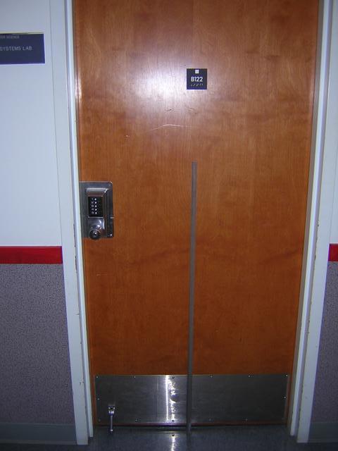 |
| The hinge we'll attach it to. It is currently attached by velcro, but will probably end up duct taped... |
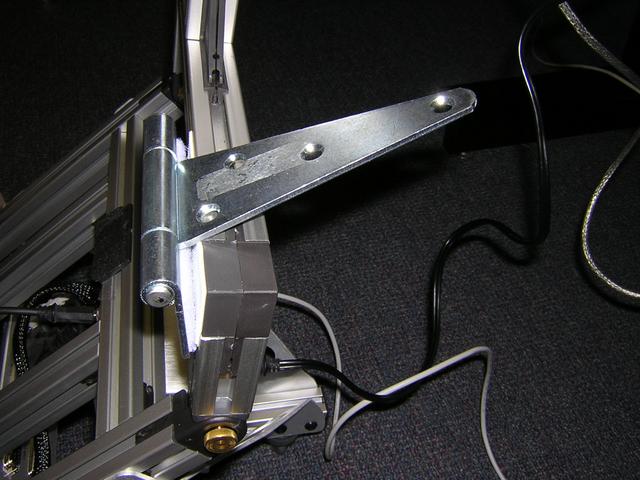 |
| The testing setup | 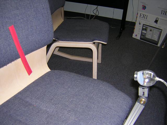 |
| The camera's view | 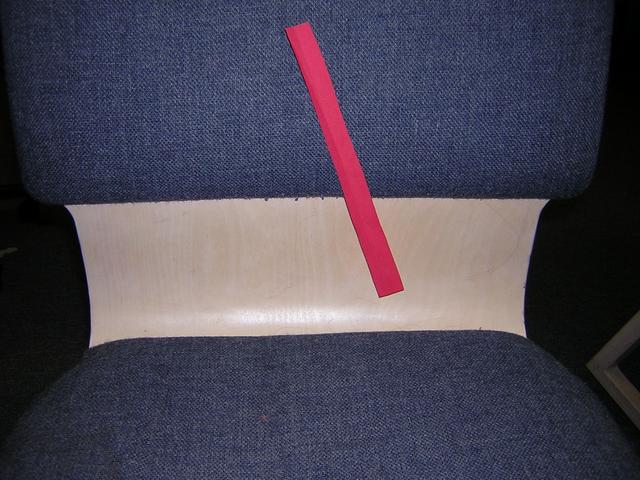 |
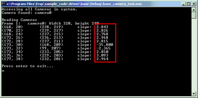
| And the result. Note that most of the slopes were close, while a few were way off. Also, our up and down are reversed, so the slope should be negative. |
 |
Bibliography
- Brooks, Rodney A. Achieving Artificial Intelligence Through Building Robots
- Dellaert, Frank et. al. Monte Carlo Localization for Mobile Robots
- Drumwright, Evan et. al. Exemplar-Based Primitives for Humanoid Movement Classification and Control
- Horswill, Ian. The Polly System
- Leonhardt, David. Subconsciously, Athletes May Play Like Statasticians
- Mouravec, Hans. PhD Thesis
- Navarro-Serment, Luis, et. al. Millibots
- Nourbakhsh, Illah et. al. DERVISH: An Office Navigating Robot
- Roy, et. al. Coastal Navigation—Mobile Robot Navigation with Uncertainty in Dynamic Environments
- Simmons, Reid and Koenig, Sven. Probabilistic Robot Navigation in Partially Observable Environments
- Vaughan, Richard et. al. Experiments in automatic flock control
- Yim, Mark, et. al. Walk on the Wild Side