Back to Top
Landmark Recognition and Location Estimation:
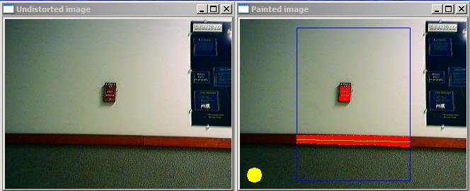
We used the Evolution's webcam to detect and extract information about
our green construction paper landmarks. The first task was to
highlight pixels which we thought were green. We did this by
empirically definining restrictions on the r,g,b, hue,saturation, and
value characteristics of a pixel. Inevitably this leaves some
noise pixels which the program thinks are green, but which are not a
part of our rectangle landmark, so we must somehow deal with these so
as to lessen the impact on later analysis. We make the assumption
that if the rectangle is being observed by the camera it will be the
largest green object in view (not an unreasonable assumption in our
leprechaun-free basement hallways). So we use a connected
component analysis to find the largest section of connected green
pixels and ignore all other pixels in later analysis. If there
are not enough
Now assuming that we do see a green rectangle in the camera's view, we
need to get an estimate of where that landmark is with respect to our
robot. To figure out its distance from the camera, we determine
the height (in pixels) of our rectangle (or blob). If it is not a
minimum height, we declare no landmark is visible (either there is no
landmark and we're looking at some other small green blob, or the
landmark is just very far away and thus too small to see
reliably). The pixel height of the rectangle, and its distance
from the camera share an inverse relationship: the shorter the distance
from the rectangle to the camera, the taller the rectangle will appear
to the camera. We model this relationship as an equation:
distance = constant / pixel_height. Theoretically this constant
would be the product of a known distance and pixel height, but we chose
to take an empirical approach to determining the constant. We
took a large set of calibration data (images and distance measurements)
and used graphing software to determine the best constant for our
equation. So using this forumula we can calculate an estimate for
the distance to the landmark. Impressively this was usually able
to estimate the distance to within plus or minus 5 cm.
Finally we had to determine the angle of the landmark from the robot's
perspective. To calculate this we determined the centroid of our
rectangle looked at its horizontal location on the camera. We
empirically determined the viewing angle of our camera, and thus
connected the leftmost column of pixels seen on the camera with the
minimum viewing angle and the rightmost column of pixels with the
maximum angle. Then for any pixel we used its horizontal location
to interpolate what angle it must correspond to. For example our
camera could see from -20 to 20 degrees, so a pixel with an x
coordinate of 50 in a 200 pixel wide window would be estimated to be at
an angle of 10 degrees (assuming positive degrees are defined to be
those left of center). Correcting for a systematic shift that
appeared, our program was usually able to estimate the angle of the
landmark to about plus or minus 3 degrees.
Here is a zip containing our modified
VideoTool, MapTool, and Wandering client.
And for those interested in the highlights, here are links to the
Wanderer, the
VideoTool source, and the
MapTool robot source.
Back to Top
Set:
The Set challenge was excellent practice in computer vision
techniques. To run our modified version of VideoTool, save
pictures of the Set game in C:\BMPs then run VideoTool.exe. Hit
'S' to load the pictures into the 12 waiting frames, then 'X' to have
Video Tool solve the problem. It will output what it believes
each card contains, then the sets that it detects. Our
Set-solving code is available
here.
Our code solves the set problem through the following
method. Each card image is sent to a processing function that
converts it from a picture to a binary matrix, where 1 corresponds to a
pixel that is likely part of the shape according to our color detection
code, and 0 is background. As this is done, the color of the
shape is determined by counting which color dominates in the shape as
the matrix is constructed. The color information is passed back
to be saved for future reference, and the binary matrix is passed on to
3 more functions to determine the number, shape, and texture of the
figures on the card.
The counting code simply looks through the matrix until it finds a 1,
indicating a part of the shape, then performs a BFS to mark the entire
shape as counted. If there are enough pixels in the shape(~450)
it is determined to be a valid Set shape. This is to help weed
out false shapes created by the similarity of certain parts of the
background to green pixels. When the code is done, it returns the
number of shapes it counted, hopefully bewteen 1 and 3.
The texture code processes the binary matrix by drawing vertical lines
through the shapes and tracking 2 important pieces of information: the
maximum number of "on" pixels, and the number of times a transition
from an "on" pixel to and "off" pixel occurred. The second piece
of information can be used to easily distinguish the striped shapes,
since they contain many transitions. Empty and filled shapes have
similar number of transitions, however, so the information on the
maximum number of "on" pixels encountered is used to differentiate the
two cases. When the function is done, it returns an integer code
corresponding to the texture it believes the card has.
The shape code draws 10 horizontal lines from the left edge of the card
to left-most edge of the first shape. The column number at which
the shape edge occurs is stored in an array. When all 10 values
have been calculated, the function analyzes how many times a transition
of more than 3 pixels occurs between two measurements. This gives
an decent overall impression of the shape on the card: ovals always
have 4(or possibly less) large transitions, squiggles have from 5 to 7,
and diamonds have 8 or 9. The function passes back an integer
code corresponding to the shape it believes is on the card.
Once all the information is gathered, the program chooses any 3
different cards and checks to see if they are either identical or
disjoint for a given attribute. It can thus easily report when a
set occurs. So far all sets tested on the current code have been
valid, so the code is deemed solid, though it is possible some
detection glitches may still exist.
Back to Top
Achieving Artificial Intelligence through Building Robots by
Rodney Brooks.
Dervish: An office-navigating robot by Illah Nourbakhsh, R.
Powers, and Stan Birchfield, AI Magazine, vol 16 (1995), pp. 53-60.
Experiments in Automatic Flock Control by R. Vaughan, N.
Sumpter, A. Frost, and S. Cameron, in Proc. Symp. Intelligent Robotic
Systems, Edinburgh, UK, 1998.
Monte Carlo Localization: Efficient Position Estimation for
Mobile Robots by Dieter Fox, Wolfram Burgard, Frank Dellaert,
Sebastian Thrun, Proceedings of the 16th AAAI, 1999 pp. 343-349.
Orlando, FL.
PolyBot: a Modular Reconfigurable Robot Proceedings,
International Conference on Robotics and Automation, San Fransisco, CA,
April 2000, pp 514-520.
Robot Evidence Grids (pp. 1-16) by Martin C. Martin and Hans
Moravec,CMU RI TR 96-06, 1996.
Robotic Mapping: A Survey by Sebastian Thrun, CMU-CS-02-111,
February 2002
Robots, After All by Hans Moravec, Communications of the ACM
46(10) October 2003, pp. 90-97.
The Polly System by Ian Horswill, (Chap. 5 in AI and Mobile
Robots, Kortenkamp, Bonasso, and Murphy, Eds., pp 125-139).
An Army of Small Robots by R. Grabowski, L. Navarro-Serment,
and P. Khosla, SciAm Online May 2004.
If at First You Don't Succeed... by K. Toyama and G. D.
Hager, Proceedings, AAAI 1997.
RRT-Connect: An Efficient Approach to Single-Query Path Planning
by Steven LaValle and James Kuffner.

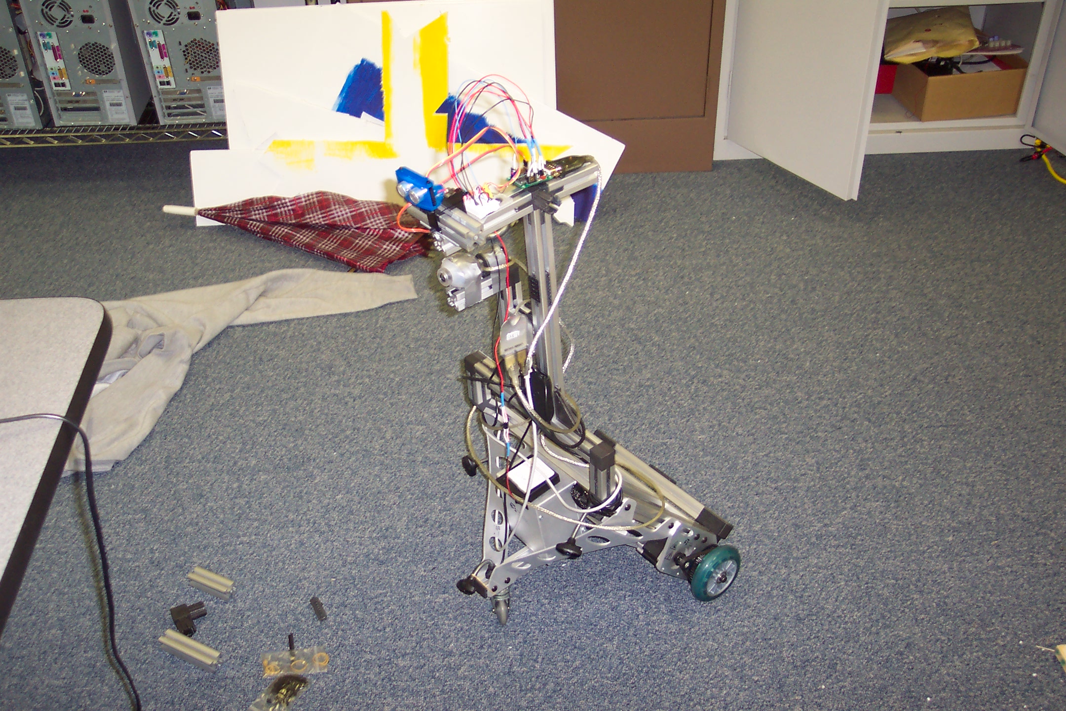
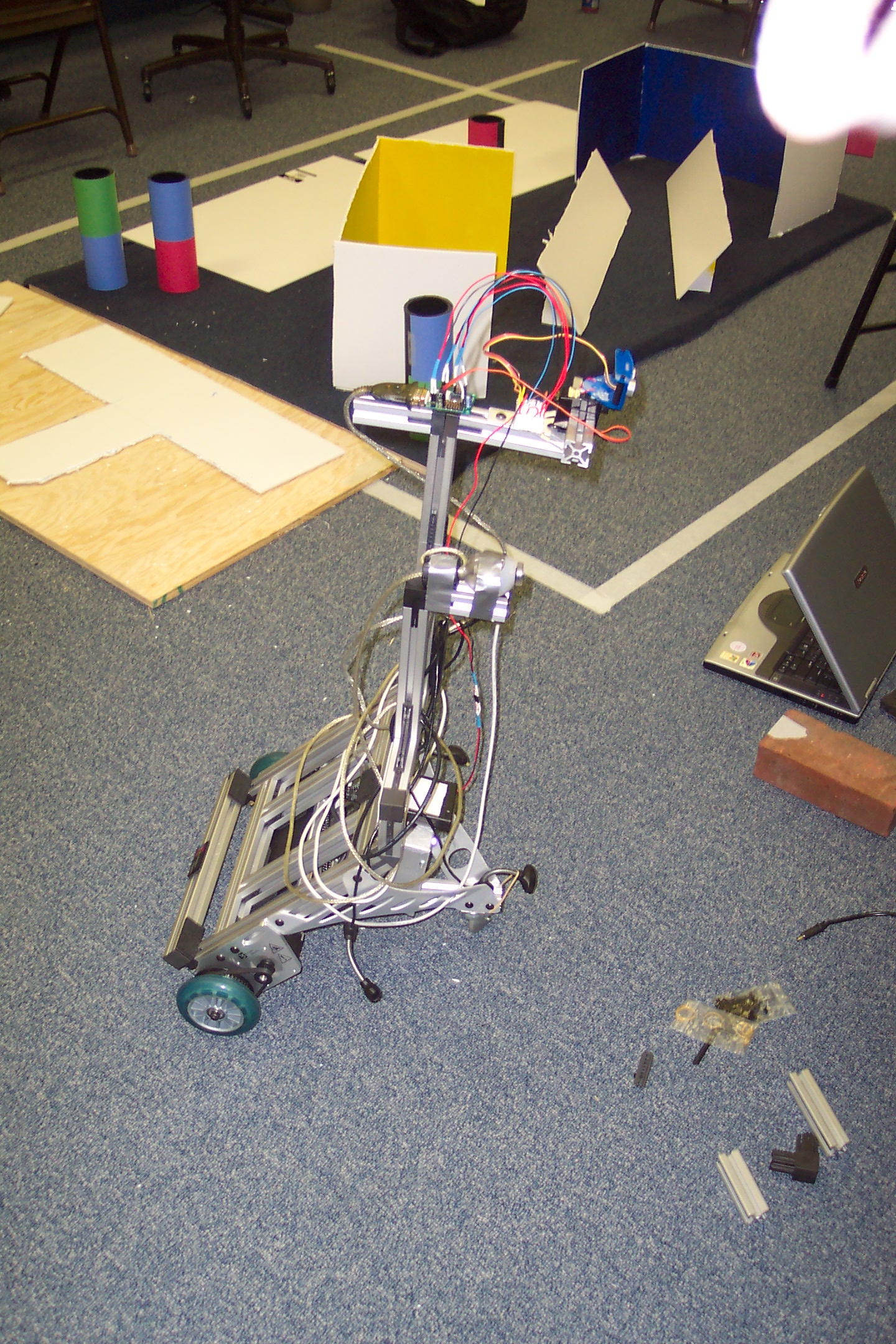
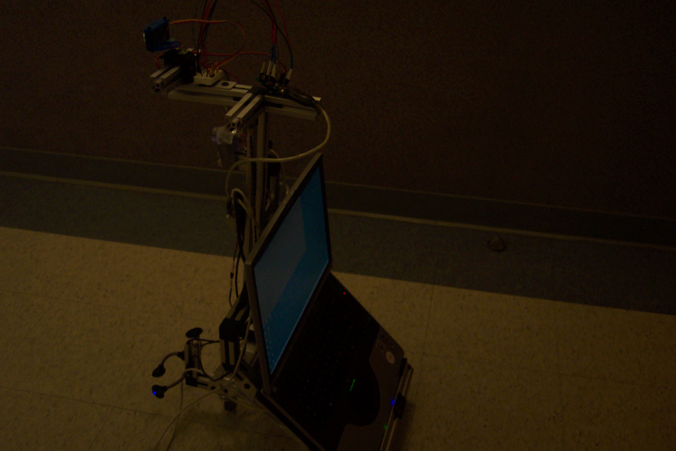
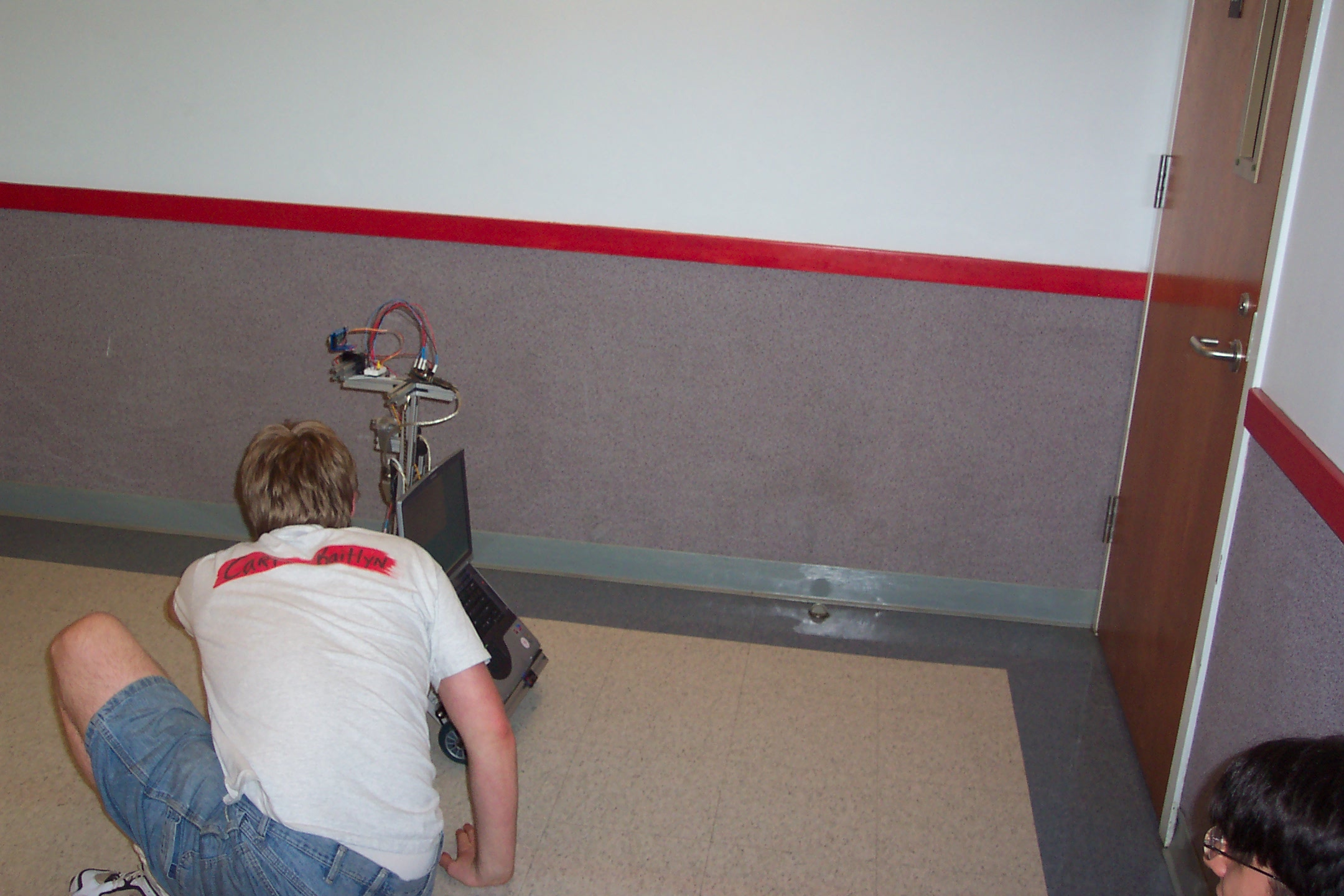
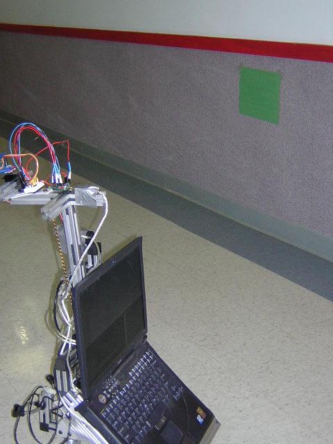 Our robot
hunting green landmarks.
Our robot
hunting green landmarks.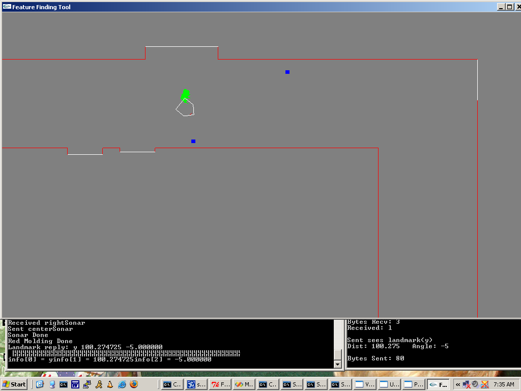 A picture of MapTool adding the
landmarks as blue squares.
A picture of MapTool adding the
landmarks as blue squares.
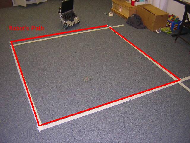 It MOVES!
 Avoiding
Stairs
Avoiding
Stairs
 Movie!