
|
|
|
|
|
We plan to make a robotic printer. It will print on the ground using either tradition paints (spray cans/pens/markers) or by dropping items on the ground (such as varyingly tarnished pennies).
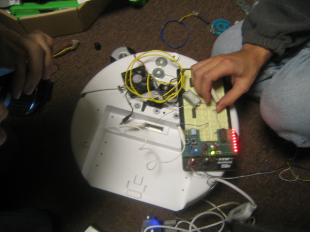
We tentatively plan to use a roomba as the base platform for our robot.
We modified our inverse kinematics from our previous update. Previously, we tried to find straight lines between the current pen position and the destination. However, in order to do this accurately, the velocity of the robot's wheels must be continuously varied. We found that trying to change the wheel speed too frequently resulted in undesirably jagged motion. To fix this problem, we decided instead to find an arc between our current position and destination that we can travel along with constant wheel speeds. We find this arc based on the fact that the robot, and thus the pen, can rotate around any point along the line defined by the two wheels. Therefor, we can always find a circle centered on this line that contains both the current pen position and the destination. To find the center of this circle, we find the intersection of the line defined by the current position of the robot's wheels and the perpendicular bisector of line segment joining the current pen position and the destination. We can then calculate the constant wheel speeds that allow us to move around this circle.
Because it doesn't require constantly changing the robot's wheel velocities, this approach allows for much smoother motion and less jagged pictures. To facilitate this, we also significantly reduced the number of points in our images. To move from point to point, we set an update delay of about 1 second. We then calculate approximately how far towards the next point we can move in the next second and choose a destination on the line between our current position and the next point. We then move to this destination using the approach described above. Our robot uses a speed parameter to determine how fast to go, but if going at its normal speed would cause it to overshoot the next point in the image, it will reduce its speed to reach the point exactly instead. After the delay time, the robot's position is updated from its odometry and a new destination is selected, until all of the points in the image have been reached. Because the odometry is not accurate for long, the robot will periodically re-localize using the vision component.
After the modifications to the vision system in the last update (optimized color identification), we decided that it would not be possible to get sufficiently accurate positions in real time. We no longer poll the vision system as fast as the robot updates, instead the robot only occasionally attempts to localize itself through vision in order to correct drift. Also, the robot uses several frames from the camera and averages the resulting positions together rather than just using a single image.
Because we no longer have to worry about real-time performance, a much more accurate computation of the position of the robot can be done. First, the image is now corrected for lens distortion, an operation which was previously too expensive to be done in real time on our laptop. Additionally, we blur the image to remove fine noise, and we subtract out a captured background so that we only consider areas that have changed since the background capture. If the robot is not included in the background capture, then as long as it is visible it will be in one of the changed regions.
Finally, we use the previous optimized selection mechanism but with one change: rather than taking the center of mass of the region matching the desired color characteristics, we calculate contours for the thresholded image and take the center of mass of the largest contour. This method is much more robust against noise, since small random noise far away from the robot's position will not affect the largest contour but will affect a global average.
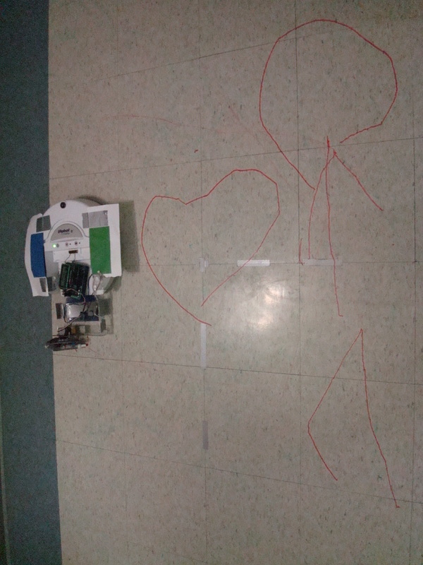
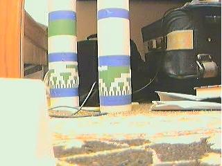
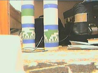
Here are a couple of pictures and a video of our system in action:
We also fixed a few bugs during our final weeks. Most notably, we added a delay for standing still before the robot gave us back odometry. This dealt with a lag we had which was causing us to draw in waves and sawtooth patterns.
Overall, I would say that our robot was a great success.
Here is our code in its final version: Final Code
Localization now uses an offboard camera. Compared to localization with posts, the task is greatly simplified. In particular, if it is assumed that the robot can only move along a plane, which is true of the Roomba, then provided that the plane is not parallel to the view vector of the camera, there is a one to one mapping between points in the camera's image and points on the plane. Hence, computing the robot's position is only a matter of detecting its position within the image and then transforming those coordinates into the coordinate system of the plane.
The actual identification of the robot is fairly straightforward based on colored markers placed on the robot itself, however optimizing the routines to reach an acceptable level of performance was not trivial. The first technique we used was to correct the image for distortion, blur it, convert it to HSV, select colored regions in it twice based on calibrated ranges, and then find the contours of the selected regions to find the markers.\ Needless to say, this was very slow, and worse, slowed down sporadically, sometimes freezing for up to a few seconds before the images updated again.
Stripping out everything, including HSV, and selecting only based on RGB yielded almost acceptable results. The video we have of directing the robot is based on this system (our camera stopped working before we could get a video of the improved system, yet to be described).
However, it was clear that just the selection task had to be optimized, and ideally the HSV conversion would be brough back into the process. The solution was to precompute a large three-dimensional table of quantized RGB values and whether they are within the selection range. The table is of the form table[r][g][b], and each entry is zero or one, specifying whether those rgb coordinates, when converted to hsv, would be within the selection range. Both the HSV conversion and selection tasks are signficantly sped up by combining them together into a table.
The actual implementation stores two entries per rgb value, corresponding to the two selection ranges for the blue and green dots, and both selections are done simultaneously to further optimize the process. The table is 30x30x30x2, or 54,000 entries; compare this to the 320x240x3 = 230,400 entries in the representation of one of the images, and the size is not so large. The table is computed very quickly; it takes far less than one second. With this method, HSV conversion and selection is significantly sped up so that the system's bottleneck becomes acquiring the image from the camera itself rather than the processing.
The second part of the vision system, transforming from image coordinates to plane coordinates, is significantly simplified by assuming that the plane can only tilt towards or away from the camera; there can be no component of the tilt that varies horizontally. Based on a tilt slider, the normal and two tangent vectors specifying the plane's coordinate system are calculated. Conversion from image to plane coordinates is then simply a matter of intersecting the line traced from the desired location in the image with the plane and projecting the 3d location on the plane thus obtained onto the tangent vectors.
In principle, the plane can also vary in distance from the camera and the camera can vary in terms of its focal length, but due to the nature of the perspective transform, the plane distance and the focal length both determine the same parameter, which is only a scaling factor.
In practice, there are two settings that must be manually calibrated: the plane tilt, and the scale (distance). The user tilts a grid superimposed on the image until it aligns with convenient parallel lines in the image, and then the user sets the scale until the grid spacing is equal to some reference mark in the environment (such as a 10cm strip of paper, or 1ft long tiles).
To control our robot's motion, we create an "image" consisting of a sequence of points that we want the pen to travel between, as well as an indication at each point whether the pen should be up or down on the way to that point. By visiting these points in succession, our robot creates a "connect the dots" picture.
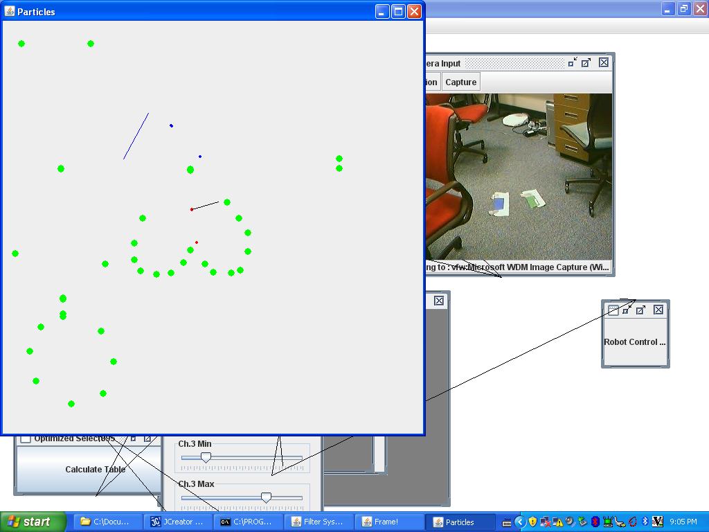
Since our objective is to move the pen along a specific path, we must solve for the inverse kinematics of the pen-robot system. To do this, we decompose the desired pen motion into a "forward" and a "horizontal" component with respect to the robot's current orientation. Moving the pen forward is simple because a forward motion of the robot corresponds to an identical forward motion for the pen. A horizontal pen movement is more difficult however, as the robot is not capable of moving sideways. However, for small angles, a rotation of the robot is equivalent to a horizontal motion of the pen by the angle rotated times the distance of the pen from the robot. Based on this decomposition, we can determine the desired ratio of forward motion to rotation, and move the robot accordingly. After a short time, we update the position of the robot and recalculate the rates of forward and turning motion. Because our images consist of a large number of points with very little separation successive points, the robot never needs to turn far on its way to the next location and the small angle approximation is valid. To determine it's position, the robot uses frequent updates from the hardware odometery, with less frequent absolute localization from the vision component. The inverse kinematics works in simulation (shown above), and has been integrated with the image processing in principle, but has not yet been fully tested with the hardware. The next step is to finish putting all the pieces together and use the inverse kinematics together with the vision to actually draw pictures
In the future, we want to get rid of the non-wireless cord. Also, we must do thurough testing and parameters setting. We also want to make it play songs and add multiple pens.
It would also be fun to guide the robot on the fly or otherwise introduce-human interaction.
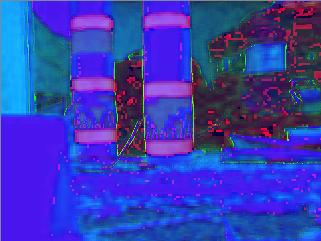
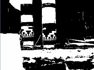
The next step is to produce two images from the HSV converted, undistorted image: a 2-bit (thresholded) image where white corresponds to the color of the blue strips on the posts, and a 2-bit image where white corresponds to light areas and black corresponds to non-white areas (either because they are too dark or they are a distinct hue).
Both of these images can be produced by running all the pixels of the image through some sort of selection mechanism that can identify pixels in the desired set (e.g., blue pixels). The simplest selection mechanism is simply an axis-aligned bounding box in HSV space: that is, all pixels that fall within a certain H range, a certain S range, and a certain V range are selected. The bounding box can then be represented with six values specifying the ranges for each of the channels; in our implementation, we also add the ability to set the minimum value of a range above the maximum value, in which case the selector selects everything outside the range (values above min OR below max [when min > max]). This is helpful for some cases, such as selecting the hue red, which, due to the HSV mapping, is both the smallest values of H and the largest values of H.
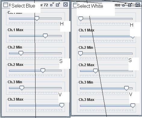
For the blue selection, the hue range is a small segment slightly to the right of the middle of the
total H range, the saturation select range is everything except the very bottom of the range (the
strips have to have at least some saturation), and the value range is everything except the bottom
(zero values produce unpredictable hues).
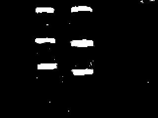
For the white selection, hue is everything, saturation is only the low end, and value is only the
high end. This selects pixels with low saturation (little difference between color channels in RGB)
and high value (high largest color channel value in RGB), which tends to select the whitest, brightest
pixels as desired.
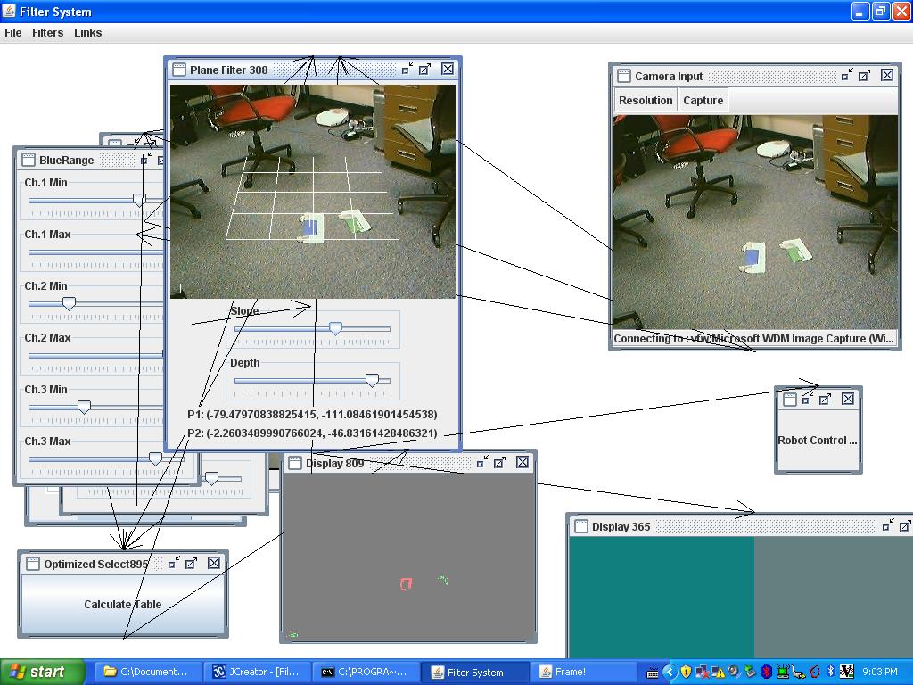
The actual ranges used must be calibrated to the lighting conditions of each test area, but the screenshot
to the right shows a set of calibrated ranges as well as the resulting images from selecting with those
ranges.
The advantage of contour selection of connected components is that, we've found, it is actually much faster in practice when compared to even an efficient (union-find based) connected components implementation. Additionally, contours can be easily used to compute the curvature of the contour, which can itself be used to help identification. With connected components alone, curvature computation would require another algorithm to do the contour selection. The disadvantage is that contour selection will select black components (which connected components does as well), but due to the nature of contours, it is not as straightforward to prune black components. The correct way to do it (which we do not, since black components [that is, black regions within white regions] occur very infrequently) is to compute the average curvature of the contour: the contour selection algorithm winds black and white regions in opposite directions, and the average curvature's sign corresponds to this winding.
Now, we know that all of our posts have three blue bands stacked vertically on top of each other, so now we search our collection of bounding boxes for 'stacks' of boxes.
We do so by first sorting the bounding boxes from top to bottom based on their top y-coordinates. Next, starting with the highest box, we look at all the boxes lower than it, in order, to see if we can find a match. A match occurs when a box is found of approximately (falling within a certain range of ratios) the same width as the target box and which is positioned approximately (within a certain range expressed as a proportion of the width) below the target box. When the first match is found, the target box has its match set to the found box, and the target box becomes the next box in the list. In this fashion, each box is matched to the closest box below it which can sustain a match. Also, note that noise will not affect the correct matching of two boxes even if that noise is between the two boxes, unless that noise is sufficiently similar to a correct match to be incorrectly matched itself.
In the screenshot in the section on reading the post's id, matching boxes are connected with white lines, and the lowest box of each stack is colored in green rather than red.
While additional constraints can be imposed, such as using the fact that the stripes occur at known positions relative to one another, selecting posts is a compromise between avoiding false positives and false negatives. Additional constraints reduce false positives by making it less likely that noise or background objects will satisfy all the constraints, but additional constraints also make it more likely that imperfections in the post, camera alignment, HSV selection, and all the other steps in image processing will cause a constraint test to be failed and falsely reject an actual post. The constraints we have chosen are already enough so that false positives are extremely rare; however, false negatives are relatively common, and we do not want to make finding posts any more difficult than necessary.
Actually reading the ID is a simple matter. Since the ID occurs between the first and second stripe, the midpoint between these two stripes is calculated. Then all the pixels (in the white-selected image) within a proportion of the stripe width (50%) and between the midpoint and the first stripe are averaged, and the result thresholded to get the most significant bit. Similarly, the pixels below the midpoint and above the second stripe are averaged and thresholded to get the least significant bit. These two bits are interpreted as a 2-bit binary number to produce the post ID.
This binary encoding was our second design, although in retrospect it is both the obvious design and the better one. Our first design was to encode the ID as simply a number of stripes, so that post ID 1 corresponded to 1 stripe, post ID 2 to 2 stripes and so on. The stripe-number encoding was extremely error prone, since it relied on scanning through the midline and counting the number of edges seen. Thus, any single-pixel noise or bands of noise that occured within the midline would result in erroneous readings. In contrast, the binary encoding is extremely robust, since the noise must be severe enough to compromise more than half the pixels in averaging region to flip a bit and cause a post ID reading error. This can occur, however, especially when reading the ID of distant posts, where there are fewer pixels in the ID region and hence less noise required to cause an error.
The distance to a post is much simpler to read: first, the height of the post (in pixels) is calculated as just the difference of the bottom y-coordinate of the bottom element of the stack and the top y-coordinate of the top element of the stack. Next, in the regular projective transformation (which we assume the image from the camera is) the apparent height of an object varies inversely with its distance. That is, h' = kh/d where k is some constant. By solving for k we find that k = dh'/h; we can then find k empirically by measuring the apparent height of an object with a known height at a known distance. Once we have calculated k (which only needs to be done once for a camera and a set of undistort parameters), we can find the distance to a post based on its apparent height by: d = kh/h'. In practice, we found the value kh for a post since we are only measuring the distance to posts, in which case the distance becomes d = (kh)/h' and kh is found by (kh) = h'd, so only the apparent height and actual distance need to be known.
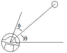
The angular position of the post relative to direction the robot is facing is similarly easy to calculate. Assume that we
know the relative angular direction of the camera to the facing of the robot, and this value is labled phi. Then, given that
we have identified a post in the image at x-coordinate (in the image) of x, we wish to calculate the relative angular position
of the post to the direction the camera is facing. [Note: we measure x-coordinates relative to the center of the image, so,
for instance, in a 320x240 image, the x-coordinate -160 would correspond to the leftmost position in the image, and 160 to
the rightmost position, and 0 dead in the center]. In the standard projective transform, we can set up a triangle where x
is the x-coordinate, theta is the angle to the post, and F is some focal length.
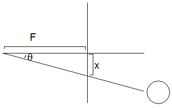
We then notice that tan(theta) = x/F, from
the definition of tangent. Now, if we knew F, we could calculate the angular position of the post by theta = arctan(x/F).
Luckily, F can be calculated empirically by measuring the angular position and apparent x-coordinate of an object, and then
calculating F = x/tan(theta).
Finally, the angular position of a post relative to the facing of the robot is just given by theta+phi [Note that this value is measured *clockwise* from the robot's facing].
The gray code is read in a different way: once the region of the gray-code has been identified, the midpoints (along a vertical
line) of the gray code bits are calculated. Then single pixels from each of those midpoints are sampled and taken to be
the bits of the gray code. No averaging can be done horizontally, since the gray code changes with the horizontal position
(we only want to read the gray code bits at the center of the band; i.e., facing directly towards the camera). However, a more
robust approach would average vertically over the entire gray code bit band height.
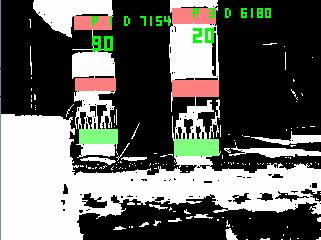
In this screenshot, components have bounding boxes drawn, and matched bounding boxes are connected with white lines. The ID of a post
is given in green text after the letter P; the distance to the post is given after the letter D, and is expressed in cm * 100
(e.g, 7154 is 71.54cm). The gray code value (out of 128) is the large number in green.
To account for the different types of readings when estimating particle probabilities, we compared the observed values with the values each particle should have seen when looking at any of the posts in our map. Determining the expected values is simple because the map consists of only 4 posts laid out on predefined locations on a rectangle. The differences between these values were used to calculate weights for the likelihood of the robot being at the location of each particle through the following basic method:
1) Initialize the particle's weight at 0
2) Find the difference (call it delta) between the measured and
expected values for post we think we've seen.
3) Normalize delta to be approximately between 0 and 1, where 0
indicates perfect agreement with expectations, and 1 indicates
complete disagreement.
4) For each delta, compute C / (1/C + delta) and add it to the
particle's weight, where C is a parameter indicating how confident we
are in the given measurement. This parameter is relatively high for
distance measurements and low for absolute angle measurements, for
example.
5) Perform the same calculation over the remaining posts that we don't
think we saw, but only add a fraction of these values to the
particle's total weight.
6) Repeat for all particles, normalize their weights, and cull and
resample the population.
Our model for modeling robot odometry was simple and based on the odometry that we obtained from the robot, namely delta distance and delta theta. We used the model from class of turning, then driving, then turning again to get to the final point. We found that both the first and second turns were equal to one half of delta turn and that the distance was d_out = (d_in * sin(theta)) / (theta * sin((pi - theta)/2)).
Tests involving synthetic data suggest that for four posts each of which has the distance measured with an error of +/- 10cm, the error in the location is also approximately +/- 10cm.
The orientation of the Roomba can also be calculated after the Roomba's position has been estimated. Suppose the Roomba sees
a post at an angle of phi clockwise from the direction it is facing, and that, based on its estimated position, the absolute
angle (measured counterclockwise from due east) of the post relative to the Roomba is theta.
 The Roomba's orientation, as measured counterclockwise from east, is given by theta+phi.
Physically, to see enough posts the Roomba must rotate the camera 180�, turn around 180� and repeat the viewing process to see the posts behind the Roomba, after which it rotates another 180� to return to its starting orientation. If the Roomba does not see enough posts in the process (it needs to see at least three), then it rotates one third of a full rotation and repeats the viewing process in the hopes of seeing more posts (it keeps the posts it has already seen in memory). When the Roomba moves it discards the posts it has seen, since those observations no longer correspond to the current position.
As can be seen from the video, in general the direct localization is good, since it determines the Roomba's position within about 10cm and the Roomba's orientation within +/- 10�. However, for the purposes of drawing pictures, 10cm is not nearly good enough to properly align parts of a drawing, and a 10� error in pose will produce severly crooked lines. Additionally, the small field of view of the camera meant that, ironically, once the Roomba got sufficiently close to a post it could no longer see enough of it to properly identify it, and the post diagonal to it was then too far away to be identified. Since the Roomba could then only identify two posts, it would get stuck in a loop of searching for more posts. Finally, the slow speed of this localization (which can be seen in the video, which is only one localization) is the colloquial nail in the coffin for on-board camera based localization; to draw a picture with any sort of complexity will require at most 1cm error and better than 1s localization times.
Theoretically, our algorithm for robot movement was to run as follows. First, wander around a bit to find out where the robot is with MCL. Then, commence the drawing of the lines. To draw a line, first attempt to drive to the beginning of the line. Once you have driven the correct distance, check your position against the beginning of the line. If you're not close enough, iteratively head towards the beginning of the line until you are. Once you are close enough to the beginning of the line, rotate yourself until you are facing the correct distance within some tolerance. Once you are oriented correctly, put the pen down and then drive to draw the line. Repeat until you have drawn the entire picture. In practice, drawing did not work well at all. In attempts to have the robot draw a square, no recognizable square was ever produced, even though the individual localizations (through direct localization) as sub-steps of the drawing process were generally correct.
To ease the creation of new pictures for our robot to draw, we created a small python application to draw pictures by clicking on the screen to draw line segments. The coordinates of these lines segments were saved to a text file which could be loaded later. Ideally, this program could factor in the offsets having to do with the pen's displacement from the center of the robot also.
After tinkering with elecromagnet and permanent-magnet based mechanisms to pick up and drop washers, we have (for the moment) abandoned the washer idea, and instead we have decided to simply have the robot draw with markers. The reason is that we could get absolutely no precision in the dropping, and the magnets had the tendency to pick up nearby washers as well.
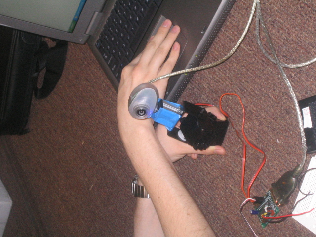
Based on the frustration of having to carry around a laptop behind the robot, we finally mounted the laptop on the robot with velcro. Additionally, we built the mechanism to lower and lift a pen or marker to allow the robot to draw. Finally, we mounted the camera on a pan/tilt servo assembly to provide the robot with the capability of looking at both the ground (the image it is drawing) and its surroundings (localization). Additionally, we wrote the servo control software.
Based on the ideas of ______ we decided to use an 'inverted' form of her tracking-beacon based localization system. Rather than having a post mounted on the robot, we will place three or more posts around the environment; each post will have a code uniquely identifiying it, as well as possibly a gray-code to indicate the angle from which it is being viewed. Combined with the distance information provided by the apparent size of the post, four different localization methods can be used.
First, with only one post, the distance and gray-code are sufficient to localize relative to that post; if the locations of all three posts are known a priori, each additional post can be used to confirm the localization estimate from all the other posts.
Next, if the pose (that is, the angle of the robot relative to the 'facing') of each post is known through the gray-code, then any two posts can be used to localize the robot by simply taking the intersection of the two lines originating from the posts and oriented in the angles indicated by the gray codes.
With three posts, knowing only the distance to each is sufficient to uniquely identify the location of the robot. In fact, with only two posts the number of possible locations can be narrowed down to only two, and only one of those can be within the triangle formed by the posts. Therefore, if the robot's motion is restricted to within the triangle, three posts provides three independent estimates of the location.
Finally, if the robot is confined to the triangle, it is not necessary to know the distance or pose of any of the posts, only the relative angular positions of the posts. This only provides one location estimate, however.
Towards these goals, we have worked on vision based identification of posts based on color. In our current test implementation, we first convert into HSV color space and select colors that are 'sufficiently close' to a sample that the vision system is calibrated to. Sufficiently close means that a histogram of HSV color frequencies is built up from the sample image, and the HSV range in which 90% of the samples fall is chosen as the selection range. This works reasonably well, but there is still significant noise to worry about. Additionally, when trying to identify the blue tape on the post, the selection only catches the edges of the tape for reasons we do not understand.
However, 'back of the envelope' calculations indicate that just based on the image size of an approximately 30cm tall id code on a post, a distance uncertainty on the order of 1cm will be possible within close distances (3m). Hopefully, a combination of all the localization methods described will be able to reduce this uncertainty, and additionally the image of the floor could be used with Monte-Carlo localization to get greater precision.
This week we got the robot to act based on information it received from the camera. Specifically, we got it to push a roll of blue tape around.
The first step was getting the robot to just follow 'light' around, by which we mean that the robot would compare the average brightness (sum of r, g, and b components) of the left and right halves of its camera input and steer to equalize them. Additionally, we programmed the robot to back up a few inches and rotate about thirty degrees clockwise whenever it hit an obstacle (its bump sensor was activated).
In the halls of Case, where the walls are not white, it was quite amusing to watch the robot steer towards the bright light of the windows. In Atwood, however, this technique did not work at all because the walls are painted with glossy white paint.
We next tried restricting the robot's view to the floor in the software by cropping out the top half of the camera input; that worked well as long as the robot did not get too close to the walls, but when it did, the blindingly white walls would enter its field of view and distract it from everything else.
Finally, we found an extremely blue roll of tape and made the robot follow only blue colors (we identified blue colors by the difference between the blue and red channels in the image); the success of this technique can be seen in the posted video. However, the robot's extremely restricted field of view (due mainly to poor mounting) meant that as soon as the roll of tape drifted even slightly to the left or right, it would leave the robot's field of vision and it would charge blindly forward.
Here is a video of our pushing success:
Here is a failed attempt:
Here's a picture of our servo-mounted camera (which we probably won't use). We can move the servos with the comptuer though.
We first went to the hardware store and bought spray paint, ten washers, and a battery. We need more washers and probably more colors of spray paint later.
We learned how to drive our actuators (wheels, speaker, LEDS, digital outputs, and low side driver outputs) from a computer. We were able to move the wheels, change the on-board LED, and drive electronics on the digital driver outputs. We have had a lot of trouble with the low side driver outputs. We also learned how to read from the web cam and the vehicle. We have yet to create a nice interface for the input and output to the robot.
Pyry Matikainen
Craig Weidert
Kevin Zielnicki