Digital Signal Processing for Music

Introduction

Sampling

Musical Signals

Fig.1

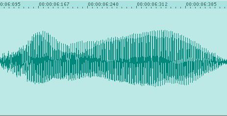
The above signal is Professor Thom on the violin playing an F#4 legato with vibrato (images are from the program DSP-Quattro). This signal is shown in the time domain, with time in seconds show across the top. It is sampled at 44.1kHz.

Fig. 2

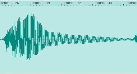
This signal is the same note, played staccato instead of legato. Looking at the signal in the time domain gives us some idea of how the volume of the note changes over time. The legato note (Fig. 1) is more or less a constant volume, with a short amount of time in the beginning where it's getting loud and a short amount of time at the end where it's dying off. The staccato note (Fig. 2), on the other hand, builds up at about the same rate as the legato note but dies off a lot faster.

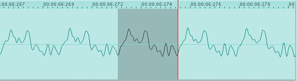
The above figures are zoomed so as to see the overall shape of the note. If we zoom in further we can see the repeating pattern of the waveform, as shown below. This is about 5 full cycles of the legato F# shown above (Fig. 1). The highlighted section shows where the signal appears to repeat. Using a different program (Matlab), we can estimate a bit more precisely how long the highlighted section is, and we find it's approximately 0.0027 seconds long. That means that the highlighted section corresponds to a frequency of approximately 1/0.0027, or 370.37 Hz. Using a chart of frequencies and their corresponding notes, we see that an F#4 is at 369.99 Hz. However, it's obvious that the note is not just made up of a single sine wave oscillating at 370 Hz. To find the other frequencies present, we have to use a process called a Fourier transform.

Fig. 3

Frequency and Fourier Transforms

When talking about the FFT, it's important to clearly define the terms used. Specifically, the input to an FFT has a number of parameters:

• fs: sampling frequency. This number is how many samples per second were taken when converting the analog signal to a digital one. It is measured in Hz. Sampling frequency is sometimes also written as f_s.
• n: the number of data points in the input.
• T: the total time we're sampling over. This is measured in seconds. It can be calculated by dividing n by fs.
• Δf: frequency resolution. This is defined as 1/T.

Our goal is to find the frequencies of the constituent sinusoids of the musical tone, because this relates to how its pitch is perceived. For the FFT to be useful, we have to have the FFT operate on a long enough time (T) so that it can distinguish between an instrument's lower pitches. The frequency resolution is the inverse of T, due to the fact that in order to resolve a frequency accurately, enough time has to pass to complete one full cycle at that frequency. For example, if we choose a T of 0.03 seconds, we have a frequency resolution of only 1/0.03 or 33.3 Hz. That's about the difference between middle C and the D above it. This means if we were using this data, for that 0.03 seconds we couldn't reliably tell if a C4 or a C#4 or a D4 was being played. Lengthening T to 0.5 seconds gives us a frequency resolution of 1/0.5 or 2 Hz, which is less than 1/8 the distance from middle C to the C# above it. However, we've sacrificed time resolution to attain this accuracy. With this T, we can distinguish only two events per second, which is too slow for our pitch detection, as the shortest notes in jazz are about 0.094 seconds long. (See Friberg and Sundström's article for more about timing in jazz.)

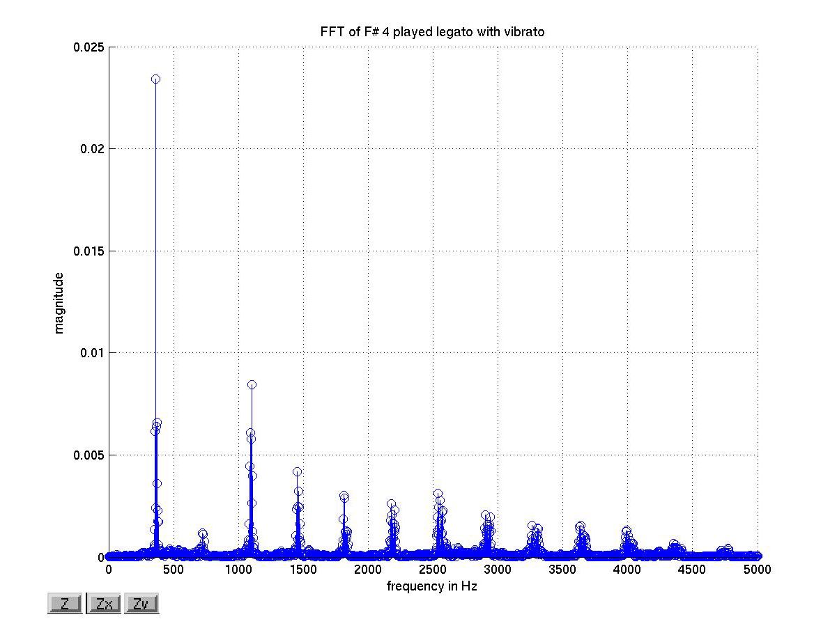
This is what the FFT of the legato F#4 (Fig.1) looks like. Frequency in Hz is on the x-axis, while the magnitude of the frequency is on the y-axis. It's drawn as a stem diagram because we have a discrete number of frequencies to represent. The FFT was taken starting at 6.095 seconds and ending at 6.440 seconds, which means our T is 0.345 seconds. Our fs was 44.1 kHz. Since n=fs*T, our n was 15214 (rounding down). Our Δf is 1/T = 2.9 Hz, but it's a bit hard to see this on the above graph. Here's a zoomed in version of the first peak.

Fig.5

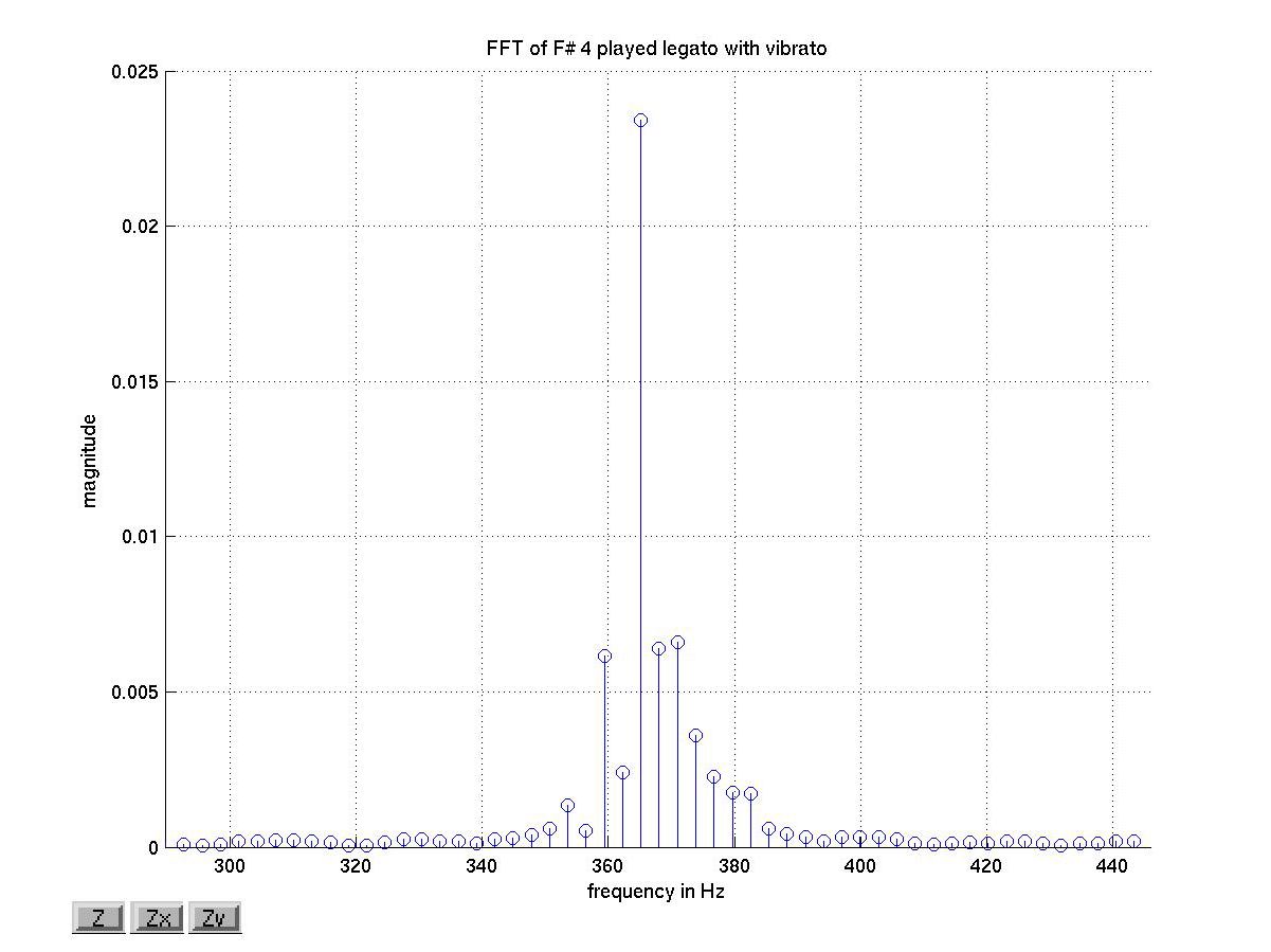
There are about seven stems in the space between 360 Hz and 380 Hz, which means that the stems are approximately 20/7= 2.9 Hz apart, just as we would expect from our Δf calculation. From this view, we can see that it looks like the tallest peak is at a little less than 370 Hz. The this peak is perhaps at a slightly lower frequency than we would expect, but the nearest notes are at 349.23 Hz (F4) and 392.00 Hz (G4), so the F#4 at 369.99 Hz is clearly the best match.

In musical sound, the lowest frequency present in a sound corresponds to the lowest order of vibration of the instrument. For example, if the note A4 at 440 Hz is sounded, the fundamental is at 440 Hz. However, the frequencies 2*440, 3*440, 4*440, etc. are also present, though most of the time they have a smaller magnitude. These other frequencies are called harmonics, and are the peaks that show up in Figure 4. The peak at about 370 Hz is the fundamental, the next harmonic is at 2*370=740 Hz, etc. Unfortunately, we found the frequency with the greatest magnitude is not always the fundamental, especially when the violin is playing a low note. For an FFT of a G3 which shows a different pattern of harmonics, check here.

Another note about the FFT is that it assumes that the sample is repeated out to infinity in order to make the math work out. For us, this means that even though we give it a segment that is 4096 samples long, it takes the FFT assuming that those 4096 samples repeat. The implications of this are discussed further on the next page.

The parameters we will use to extract pitch from the .wav file are listed below. Note that a time interval of 0.093 seconds corresponds to 16th notes played at 160 beats per minute. Windowing and overlap are discussed on the next page.