This project set out to explore the application of genetic algorithms to the weights of a neural network as a substitute for training algorithms in recurrent neural networks. Training methods for Recurrent Neural Networks (RNNs) are especially interesting because the vanishing gradient problem tends to make backpropagation unusable. Many training methods have been applied to RNNs, including Backpropagation Through Time and Simulated Annealing to name a few (see [4]). Each method comes with its own set of drawbacks, so alternative methods are an active area of research. Genetic algorithms have already recieved some attention in this area; for examples, see references.
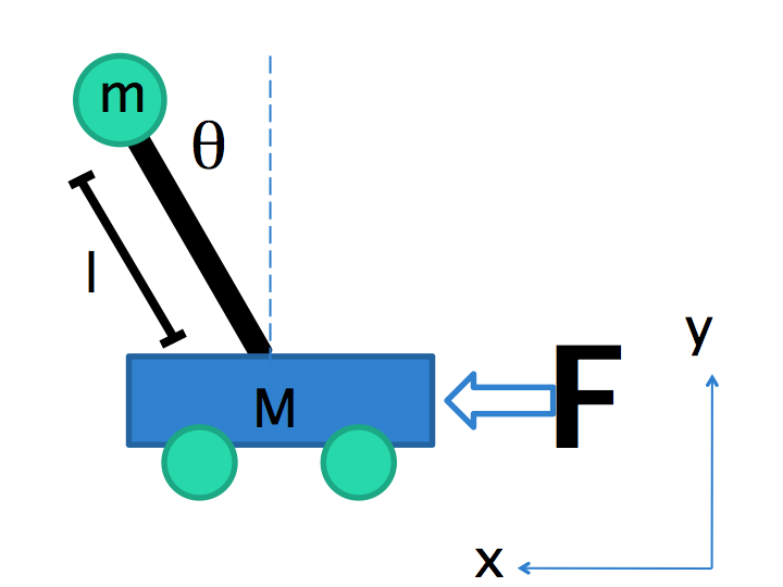
To test and demonstrate the capabilities of a RNN trained with a genetic algorithm, I chose to use the algorithm to find the optimal weights for balancing a pendulum on a cart.
The final goal of the project was to evolve a network that could balance a pendulum by outputting the force to apply to the cart at each step, given only the angle of the pendulum as input.
In order to let the algorithm find the absolutely optimum solution, very few presuppositions were made about the structure of the network. All networks started as fully connected directed graphs, though some weights were randomly set to zero so that lack of connection would be present in the gene pool. The idea was that if lack of connection gave a network a fitness advantage, it would be selected for evolutionarily. The network did follow a general forward-propagation; there was a predetermined order in which the node outputs were calculated based on the nodes they were connected to, so that some of the nodes were sharing their previous time step output and some nodes were sharing their current time step output.
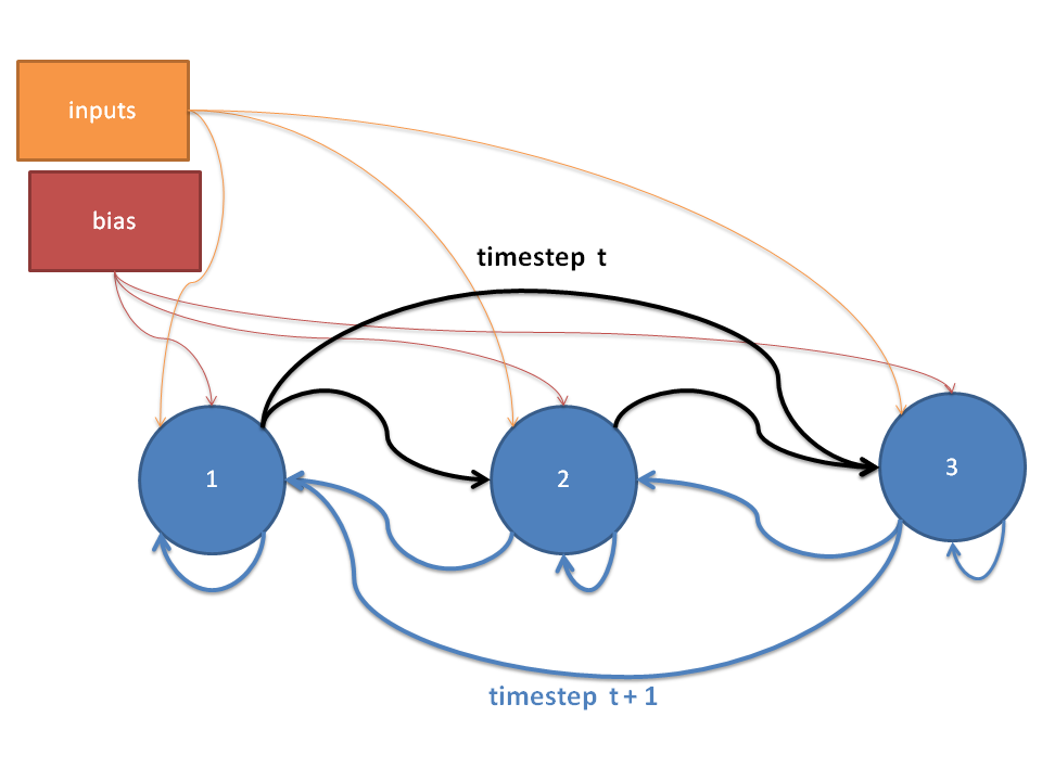
For example, in the figure above, a single forward propagation begins with node 1. The black arrows represent connections in the forward propagation direction, and the blue arrows represent feedback connections. The output of node 1 at timestep t is an input to nodes 2 and 3 at timestep t, and the output of node 2 at timestep t is an input to node 3 at timestep t. At timestep t+1, the output of nodes 1,2, and 3 from timestep t are all inputs to node 1, while only the output of nodes 2 and 3 from timestep t are inputs to node 2 at timestep t+1, etc. This can of course be genralized to larger networks.
Again, the supposition was that if having layers was advantageous, then the weight of the input between two sequential nodes would evolve to zero, so they would not rely on each other's current time step output. For example, in the figure above, we can imagine that setting the black arrow between nodes 1 and 2 would eliminate the time t input to node 2; this is equivalent to having nodes 1 and 2 in the same layer. This ended up happening at least once in the fittest anlge-input-only network, as seen below.
All nodes in the network had a bias and the external inputs as inputs to the node. The one restraint imposed on the networks was that the output node was consistently chosen to be the second-to-last node in the forward-propagation; this was an accidental choice based on an indexing error that was not caught until very late in the project. Though originally the intention was that the last node in the forward-propagation would be the output, the networks were fully functional with the second-to-last node as the output node, so there did not seem to be a need to correct the mistake.
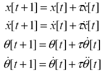
One of the initial challenges faced was accurately modelling the motion of an inverted pendulum. In [2], I found equations of motion for the pendulum and more importantly the suggestion to use Euler's method to model them linearly. The equations for the second derivatives of angle and position at time t are as follows:
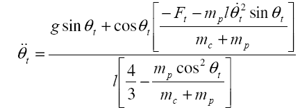 ,
,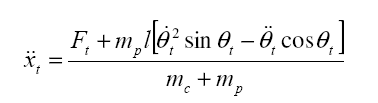 ,
,
And the angle, angular velocity, position, and linear velocity
are approximated numerically by Euler's Method:
As it turns out, there is an exact solution to this problem which depends on the angle, angular velocity, x coordinate and the velocity of the cart:
where the k_i's are constants dependant on the system.
This means that given all four inputs, it is possible to balance the pendulum with a single neuron [3]. However, the challenge of this project is to balance the pendulum using only the angle or only the angle and angular velocity as inputs, allowing the network to exploit its feedback mechanisms to deduce the angular velocity in the first case and take into account its position and velocity of the cart in both cases using the current state. Using only the angle as an input is a goal is discussed in [3], and this source acknowledges that this is a challenging problem, though the authors report very good results.
Each organism's genome was a list of floats representing the weights
of connecting edges between each node in the RNN; because the
weights are not bi-directional, each list of weights contains a
weight for the edge (i,j) and
the edge (j,i) for every node
i and every node j.
The starting population in the algorithm was generated by
creating a random genome as follows:
For each connection between two nodes:
Mutation was performed by probibalistically selecting between 1 and 3 locations in the genome and adding a random number in the range (-1,1) with increments of 0.1 to the weight at that locus.
I implemented and tested two kinds of recombination operators. The first was traditional uniform crossover, in which several indices are chosen identically from the genomes of the parents, and are then swapped. I found that randomly choosing about half the genes and swapping those genes with 0.5 probability was most effective; an expected 25% of the genes were swapped each time, but the actual percentage varied between 0% and 50%. Using a lower expected percentage did not produce children different enough from the parents, slowing down the evolutionary process.
The second method I implemented was similar to uniform crossover, but instead of swapping genes at the selected loci, the average value of the genes at that location was inserted into the genome. Although this is not a standard genetic operator, my idea was that if both parents are fit, a value between two weights at a particular edge was likely to be optimal.
After testing both operators, I decided to use uniform crossover as my recombination operator, because I found that the second method quickly eliminates genetic diversity in the population; genetic diversity came only from mutations, which made for very slow evolution.
Initially, the fitness function I used measured the number of time steps between the time at which the angle of the pendulum first arrives at 0 degrees until the angle dips below 90 degrees. This fitness function was not very effective for several reasons. For one, it does not allow the network enough time to establish balance before beggining to evaluate the fitness. Also, there is no penalty for larger angles; a network that manages to keep the pendulum between -90 and 90 degrees for the entire time interval is equal in fitness to a network that balances the pendulum perfectly.
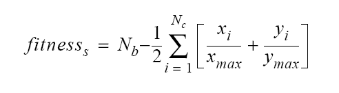
In [1], I found a fitness function from a similar application that looked promising. The author waits a number of time steps for the network to come to equilibrium, then sums the number of steps for which the network is able to keep the pendulum between -90 and 90 degrees, but subtracts at each time step a penalty for the position of the pendulum away from equilibrium:
I implemented a variation of this fitness function, in which I imposed a penalty based on the angle rather than the x and y coordinates of the pendulum:
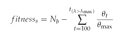
I also started evaluating fitness after 100 timesteps rather than immediately following the first occurrence of θ = 0, to allow the network to stabilize before penalizing for lost balance.
When performing evolution, I used between 7 and 10 nodes, as [1] seemed to indicate that more than 5 hidden-layer neurons were necessary (though this does not really apply to my model) and [3] seemed to indicate that 10 nodes were employed successfully for balancing the pole with angle-only input. Each organisms's fitness was evaluated with initial pendulum angles of ±10, ±20, ±60, and ±100. The fitness was evaluated starting at timestep 100 and until balance was lost or 200 additional timesteps had passed.
I initially experimented with the mutation rate and survival rate, and found that the best results were given by a mutation rate of 0.6 and a survival rate of 0.4. However, I do not have rigorous experimental results showing that these are the optimal parameter values, because each run of the genetic algorithm was highly time consuming and I did not have the time in the scope of the project to run extensive tests.
I also found that a population size of 75-100 was most successful in consistently yielding high-fitness organisms. Smaller population sizes sometimes yielded highly fit organisms, but sometimes the organisms froms small populations evolved very slowly. I concluded that a small number of organisms restricts the gene pool too much and makes fitness values too erratic and more easily dominated by a single organism, so I chose population sizes in the range of 75-100, though the larger population took far longer to compute.
I did succeed in performing 5 experimental runs in which I evolved networks of sizes 5,7, and 10 nodes in population sizes of 25, 50, and 75, for 100 generations, the results of which are summarized in the table below.
| Population Size | Number of Nodes | Average % Fitness | Minimum % Fitness | Maximum % Fitness |
| 25 | 5 7 10 | 12 17 12 |
5 8.5 0.7 | 17 20 25 |
| 50 | 5 7 10 | 13 24 20 |
1 2 17 | 21 55 21 |
| 75 | 5 7 10 | 16 20 17 |
2 19 3 | 20 21 20 |
Though there are only 5 data points for each category, it is clear that the genetic composition of the initial population is very important in determining the fitness of organisms 100 generations later. This is especially evident from the spread between the maximum and minimum fitness in each case; runs under identical conditions can produce in one case organisms with only 2% fitness, but in another case 55% fitness. Other apparent trends would need more data for support, but the maximum and minimum values can only increase in their maximality as more runs are added.
This seems to suggest that in order to evolve a really fit network without modifications to the algorithm, many runs of the algorithm with a relatively large initial population are necessary.
I found that from running the genetic algorithm for as many as 500 generations, the highest fitnesses achieved were on the order of 60% of the total possible fitness. I decided to interfere in several ways to try to induce the evolution of fit organisms, some of which were more successful than others. These techniques are summarized below:
Directly below is the schematic of the fittest network produced that takes only angle as input. Its evolution took about 500 generations. It is capable of balancing the pendulum within about ±45 degrees for extended periods of time given starting angles between -60 and 60 degrees
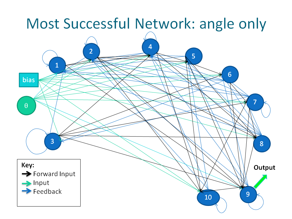
Note that nodes 1 and 3 are arranged in a "layer."
Videos of this network and its earlier ancestors balancing pendulums are shown below.
This video demonstrates that the network cannot balance when then pendulum starting position is at 80 degrees. This is true for all angles larger than 60 degrees.
It is interesting to compare the fittest network to an earlier ancestor of the network, as seen below. The amount of fitness acquired in just 100 generations is very impressive!
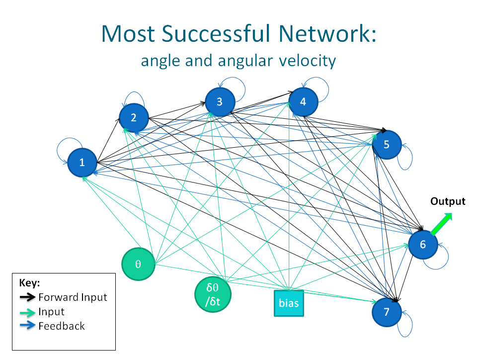
Below is a diagram of the fittest network evolved that takes in angle and angular velocity as inputs. It took about 600 generations to evolve. It is capable of completely balancing the pole given any starting angle.
Videos of this network and its earlier ancestors balancing pendulums are shown below.
The fitness of the network with angle and angular velocity as input is obviously much greater than the angle-only input network. Clearly, balancing with a single input is a harder problem. However, it is possible that the fitness of the single-input network can be further improved in successive generations of evolution; the difference in the fitness of the fittest network and its ancestor is encouraging to this end.
It is interesting that for both fittest networks, the network architechture is probably very different from anything a human being whould have designed. Although it appears that the graphs are fully connected, there are several connections missing. Furthermore, there does not seem to be a high occurrence of layering; only in the angle-only instance were the nodes better formed in a layer, and even in this case there is only one "layer" in a graph of 10 nodes.
The genetic algorithm was able to evolve networks that balance the pendulum relatively well; this is especially true for the angle and angular velocity input network, which is able to completely stabilize the pendulum starting from any angle between 0 and 360 degrees. The angle-only input network also achieved a relatively impressive level of fitness, given the acknowledged difficulty of the problem in the literature (see [3]).
I suspect that my results could be improved in a variety of ways. In references that I read, several modifications to the genetic algorithm and the network architecture were suggested that I found intriguing, but was unable to pursue due to time constraints. Furthermore, suggestions from my peers and professor and queries that have arisen in my research are also worth investigating. They include:
I would like to acknowledge Professor Keller for his advice and ideas throughout the project.
[1] Syed, Omar. "Applying Genetic Algorithms to Recurrent Neural NetworksBelow is a link to my python code for the evolution of network weights and the visual simulation of a pendulum on a cart. VPython is required for running the simulations.
GeneticRNN.pyInstructions for performing evolution or running a demo can be found at the top of the code file.
It should be noted that others experienced difficulties when attempting to perform evolution on their computers. No problems have been experienced when running the simulations on other computers. It seems as though the problem has at present been corrected, however, this has only been tested on one computer other than my own.