Lab 4: Part of Speech Tagging

Introduction

This week, you’ll spend some time working with a Hidden Markov Model Part of Speech tagger. Rather than implementing it from scratch, you’ll just add a few key lines and make a series of modifications to the tagger. Along the way, you’ll analyze the impact of different configuration settings on the tagger’s performance.

This lab will also make heavy use of the numpy package. Numpy is a very popular Python package designed to provide fast and efficient matrix and linear algebra operations using a MATLAB-like syntax. Some of you may have previously used numpy in another class, internship, or research. But if you've never seen Numpy before, I encourage you to take a quick read through the Numpy beginners' guide and make sure you understand the basic concepts and syntax. And remember: in addition to the course staff, your peers are also a resource if you need help!

Hint: Even for numpy "experts", it can be easy to lose track of the meaning of different array dimensions, and we can often still find ourselves surprised by the result of a matrix operation that doesn't do what we wanted it to. I often find it easier to "draft" my numpy operations by making some simple, small test matrices where I can check that operations are going in the direction I expect and resulting in the appropriate shapes and values. Doing these tests in IPython (or using a breakpoint in your code with ipdb) might seem like more work, but it can often make writing the correct line much faster.

Lecture Recap

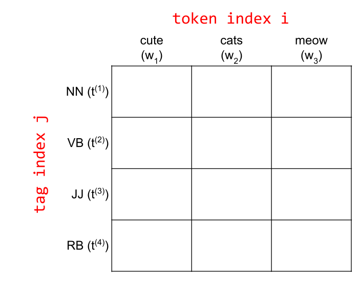
In the Week 5 lecture, we explained the Viterbi Algorithm, a dynamic programming approach for finding the most likely part-of-speech tags for a given document (token sequence). As a dynamic programming algorithm, it works by filling in a DP table (matrix) which we call \( D \). The rows and columns of \( D \) are as follows:

• Each column index \( i \) represents \( w_i \), the \( i \)th token in the document.
• Each row index \( j \) represents \( t^{(j)} \), the \( j \)th part-of-speech tag in the list of possible tags.

To keep your indices straight, it may be useful to refer to the following image, which depicts the DP table you filled out on the example worksheet, with the axes explicitly labeled:

The base case is the leftmost column, \( i = 1 \), where we filled each cell according to the following formula:

$$ D_{j,1} = P(w_1 \mid t^{(j)})P(t^{(j)} \mid < \text{SOS} >) $$

For all other columns, the key insight was that we build up the DP table from left to right, "accumulating" the calculation so that, for each column, we only need to refer to the previous column. The general formula for filling in each cell \( (j, i) \) therefore becomes:

$$ D_{j,i} = \text{max}_{j' = 1}^{N} P(w_i \mid t^{j}) P(t^{(j)} \mid t^{(j')}) D_{j',i} $$

(Where \( N \) represents the total number of possible tags—in other words, the max we are taking is a max over all possible tags.)

Implementing Viterbi With Matrices

Notice that the above calculation requires keeping track of two types of probability:

• \( P(w_i \mid t^{j}) \): This is a probability that a given part-of-speech tag will produce, or "emit", a given token (For example: given that the 3rd token is a verb, what is the probability that the token itself will be the token "meow"?). We call this an emission probability.
• \( P(t^{(j)} \mid t^{(j')}) \): This is a probability that a given tag will be followed by some other tag (For example: given that the current token is tagged as a noun, what is the probability that the next token will be tagged as a verb?). We call this a transition probability, since it represents the likelihood of transitioning from one state (tag) to another.

This is all well and good if we're doing the math on the whiteboard...but if we're implementing this in code, how do we actually keep track of the probabilities?

In practice, we store both the emission probabilities and transition probabilities as (separate) matrices:

• \( A \) is an \( N \times N \) matrix that stores the emission probabilities, such that \( A_{j',j} = P(t^{(j)} \mid t^{(j')}) \).
• \( B \) is an \( N \times V \) matrix that stores the transition probabilities, where \( V \) is the vocabulary size. Note that the indexing here is a tad more complicated. \( i \) is an index into the document, but what we need here is an index into the vocabulary. For the purposes of this lab, you don't need to worry about this; we implement the translation logic for you. So tl;dr: letting \( \text{index}(w_i) \) be a "magic" function that looks up the index of token \( w_i \) in the vocabulary, then \( B_{j, \text{index}(w_i)} = P(w_i \mid t^{j}) \).

With these matrices defined in this way, the formula for filling in the DP table becomes:

$$ D_{j,i} = \text{max}_{j' = 1}^{N} B_{j,\text{index}(w_i)} A_{j',j} D_{j',i-1} $$

One last note: during the in-class exercise, you hopefully observed that the probabilities get smaller and smaller as we go deeper into the table. In real life, the probabilities would become so small that they would lead to floating-point errors! To prevent this, when implementing the algorithm in code, we typically work in log space. This is because the log of a small probability is a big negative number (which is less at risk of overflow). The main thing to keep in mind, when working in log space, is that multiplication becomes addition and division becomes subtraction. So, the above equation becomes:

$$ D_{j,i} = \text{max}_{j' = 1}^{N} \log(B_{j,\text{index}(w_i)}) + \log(A_{j',j}) + D_{j',i-1} $$

(When logged in, completion status appears here.)

Go to Parent Page Next Page