A Biological Inspiration
Here is a diagram of a human neuron, courtesy of Wikimedia Commons:
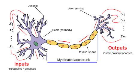

(Sound of shuffling pages) Ah yes, as a human with a brain, this looks quite right to me.
Without going too deep into biology (which we're not really qualified to do anyway), a very simplified explanation of what happens in the brain is that the neuron receives electrical signals from surrounding neurons (those signals are labeled \( x_i \) in the diagram), and if the total input voltage gets high enough, the neuron "activates" and emits signals of its own (the \( y_i \) in the diagram).

Maybe don't go showing that paragraph to the biology department; they'll probably chew us out for telling you lies about the brain.

Nonetheless, this simplified model was good enough for some computer scientists in the 40s and 50s...
From Neurons to Perceptrons
Back in the mid-20th century, scientists and engineers were becoming increasingly interested in whether this newfangled technology called the "computer" could be used to simulate human thought. Given that thought happens in the brain, and the brain is made up of neurons, developing an artificial neuron seemed like the natural first step.
Enter the perceptron (once again, thank you to Wikimedia Commons for the helpful diagram):
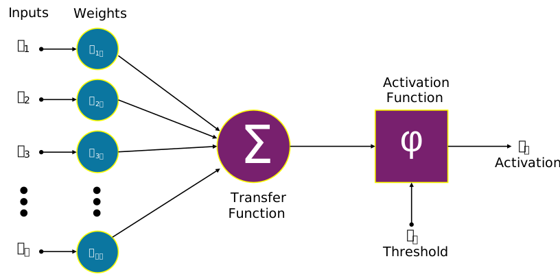

Oh yeah, comparing this picture to the previous one, I can totally see the family resemblance!

It's a loose resemblance though. Like, not twins, more like second cousins who, if you know they're related and you squint, you can kinda see it.
The perceptron is an extremely rough approximation of the (already simplified) neuron model we saw at the top of this page. It would be most accurate to call the perceptron a model that is inspired by the neuron, rather than a true implementation of an artificially simulated neuron.
It works as follows:
- In the absence of other "neurons", the perceptron takes external inputs for its \( x_i \)'s. These could, for example, be pixels in an image. More generally, we call the inputs to the perceptron features (which should be sounding very familiar!)
- The perceptron then multiplies each feature \( x_i \) by a corresponding weight \( w_i \), and takes the sum of the products (i.e., it computes a weighted sum of the features). Then it takes this weighted sum and adds a bias term \( b \).
- If the weighted sum plus bias term (from the previous step) exceeds some threshold, the perceptron is considered "active" and its output is 1. Else, it is "inactive" and its output is 0. This thresholding is an example of a more general concept called an activation function.
-
Be careful! In previous lessons we've used the notation \( w_i \) to refer to tokens (words) in a sequence of tokens, but here instead we're using it to refer to weights in the perceptron!
Of course, you may wonder where the weights \( w_i \) come from. It turns out there is a (surprisingly simple) perceptron learning algorithm that can be used to train the weights. However, we won't be covering it, mostly because it's generally considered pretty bad—it only took a few years for the research community to come to a consensus that the perceptron was more an intellectual curiosity than a practically useful model. Nonetheless, we bring up the perceptron because it serves as the foundation for other, more useful concepts we'll actually cover in this lesson.
One useful property of the perceptron that we want to establish: it turns out to be a convenient example of a linear model. But what exactly makes it linear? Well, let's think about what it actually does to the inputs: it computes a weighted sum and adds a bias. Mathematically, we might write this as:
$$ \sum_{i=0}^k w_i x_i + b $$
Where \( k \) is the number of input features. But is there a different way we could express this?

Hmm, I swear I've seen a "sum of products" like that before. I think it was sometime in Core?

Oh no, please don't give me flashbacks to Core...
Suppose we defined a vector \( \mathbf{w} \) that contains each of our weights \( w_i \). Likewise, let's define a vector \( \mathbf{x} \) that contains each of our features \( x_i \). Then, hopefully you remember from linear algebra that the "sum of products" is actually the dot product, so the above formula can be rewritten as:
$$ \mathbf{w} \cdot \mathbf{x} + b $$
And again, if you think back to your linear algebra, you should recognize this as the general equation for a line (or a plane in 3 dimensions, or a "hyperplane" in more than 3 dimensions). That's why the perceptron is a linear model...and in fact, all linear models can be expressed as a dot product plus a bias term.
The last step in the perceptron algorithm is to apply a threshold to decide whether the final output should be 1 or 0. This is actually a specific example of a more general concept known as an activation function: a function \( f \) that is applied to the sum above to map it to some finite output range. So the final perceptron output is:
$$ \hat{y} = f(\mathbf{w} \cdot \mathbf{x} + b) $$
-
The little "hat" above \( y \) here is a conventional mathematical notation for saying that this is an estimate of the true label \( y \).
For the remainder of the discussion on this page, we'll think of \( f \) as a simple thresholding function, but we're purposely using the more generic notation to remind you that \( f \) could be any activation function (which will become relevant on the next page).
Perceptrons as Classifiers
Keeping for the moment the assumption that \( f \) outputs 1 or 0, it starts to become clearer how the perceptron can be used to implement the idea of classification that we discussed in class.
Remember that \( \mathbf{x} \) is a vector of our input features. As discussed in lecture, a feature in NLP could be, for instance, the frequency of a particular token, or it could be some other property of the input text (e.g., the length of the text, or whether or not it's in all caps). Assuming we already have some weights \( w \), we can run the above formula to get an output \( y_{out} \), which will be 1 or 0. We may then treat this as the answer to a yes or no question, like "does the text have positive sentiment"?

Ok, I can see how this would work if there's only one class we care about. But what if we're trying to classify text into multiple classes?

Yeah! Like, does this recipe describe breakfast, lunch, or dinner? That's 3 classes! And we all know MORE classes are better!
For more general classification, where we may have a set of \( n \) classes \( C = \lbrace c_1,c_2,\dots,c_n \rbrace \), we would need to ask \( n \) yes-or-no questions of the form "does this text belong to class \( c_j \)?". And since one perceptron can answer one yes-or-no question, it follows that we would need \( n \) perceptrons.
-
See? I told you MORE is better!
-
You know what? For once, I can't argue with that.
-
Meh. I can argue with it. \( n \) perceptrons sounds like a lot of vectors to be keeping around!
If we think about how we would actually implement this in code, things start to get very messy very fast as the number of classes gets large. Each perceptron is effectively defined by its weight vector \( \mathbf{w} \) and its bias term \( b \). So for a \( n \)-class classification problem, the psuedocode seems to look something like this:
let x = a vector of input features
let ws = a list of n weight vectors
let bs = a list of n bias terms

let results = an empty list of size n

for j from 0 to n:
    let weighted_sum = dot_product(ws[j], x) + b[j]
    set results[j] = activation_function(weighted_sum)
This is not...terrible, exactly, but keeping around a giant list of weight vectors and bias terms seems annoying (and remember, we haven't even talked about how we learn the weights and biases in the first place!). More importantly, if you went to the math department and showed them code that's doing a bunch of dot products in a loop, they might look at you a bit funny...and that's because there's actually a more mathematically elegant way to express the logic above.
A More Elegant Implementation
-
Before we start on this, let's see if we can jog your linear algebra memory a bit.
-
Noooo! I told you not to give me Core flashbacks!
One fun linear algebra fact (which you may or may not remember) is that matrix multiplication is a generalization of the dot product! Let's quickly go over the connection, in case you need a reminder (or legitimately never learned this fact).
-
Feel free to skip this bit if you already know this mathematical property.
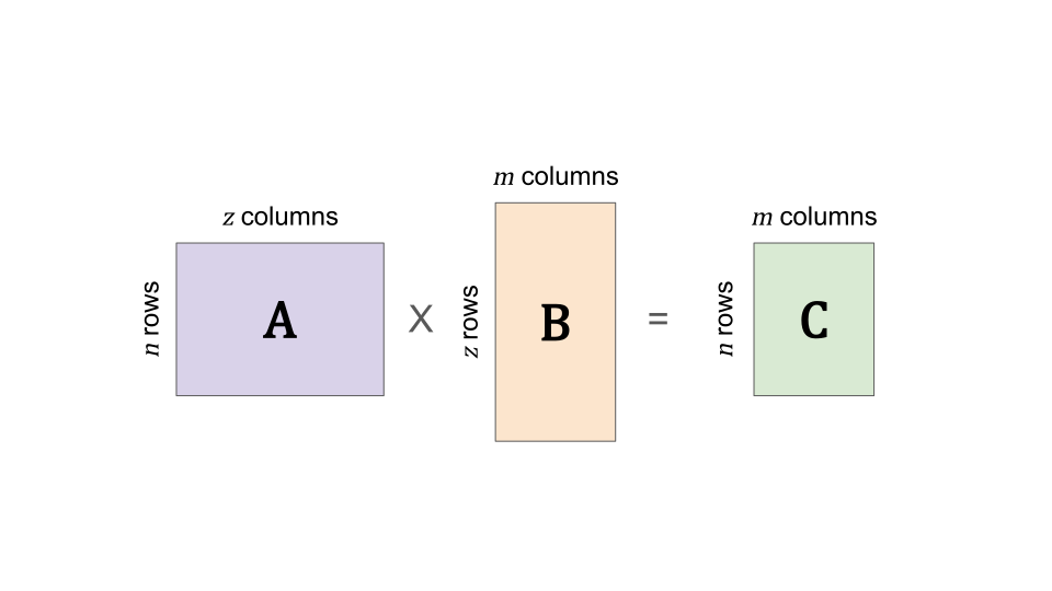
Suppose we are trying to multiply matrices \( \mathbf{A} \) and \( \mathbf{B} \). Let \( n \) be the number of rows in \( \mathbf{A} \), and \( m \) be the number of columns in \( \mathbf{B} \). The multiplication is only possible if the number of columns in \( \mathbf{A} \) is the same as the number of rows in \( \mathbf{B} \); let's call that number \( z \). The result you'll get is a new matrix \( \mathbf{C} \) with \( n \) rows and \( m \) columns.
-
Here's a handy picture to help you get all the variables straight:
You probably learned a procedure like the following to do the multiplication by hand:
- To compute the term in the \( i \)th row and \( j \)th column of \( \mathbf{C} \)...
- ...multiply each element in the \( i \)th row of \( \mathbf{A} \) by the corresponding element in the \( j \)th column of \( \mathbf{B} \)...
- ...and add up all the products you got in step (2).
But notice that step 3 looks a lot like a "sum of products"! Indeed, another way of interpreting this calculation is that the \( i \)th row of \( \mathbf{A} \) and \( j \)th column of \( \mathbf{B} \) are both vectors, and that steps 2 and 3 are just a long way of saying "take their dot product". In other words, the whole procedure can be rewritten as follows:
- To compute the term in the \( i \)th row and \( j \)th column of \( \mathbf{C} \)...
- ...Take the dot product between the \( i \)th row of \( \mathbf{A} \) and the \( j \)th column of \( \mathbf{B} \).
From this, it follows that "do a bunch of dot products in a loop" is actually equivalent to doing a matrix multiplication!
-
If you were skipping the math because you already know it, here is where you should start paying attention again.
Let's return to our classifier pseudocode. We want to replace that loop with a single matrix multiplication. Instead of a list of weight vectors, let's define a weight matrix \( \mathbf{W} \). \( \mathbf{W} \) has \( n \) rows, where the \( j \)th row contains the elements of weight vector \( \mathbf{w}_j \) in our original list. So if our input feature size is \( k \), the size of \( \mathbf{W} \) is \( n \times k \).
Then, imagine that the input feature vector \( x \) is represented as a column vector. A column vector is just a vector that's been written vertically, so that it's equivalent to a matrix of size \( k \times 1 \). Then we can see that the following matrix multiplication effectively computes all the original dot products:
$$ \mathbf{W}\mathbf{x} $$
Which will produce a \( n \times 1 \) column vector, representing each weighted sum we would have gotten from the loop. Of course, we still need to do the step of adding the bias terms. But that can just be a simple vector addition if we similarly define a column vector \( \mathbf{b} \) containing each bias term \( b_j \). So the entire loop (including the dot product step and bias addition step) can be written as one mathematical calculation:
$$ \mathbf{W}\mathbf{x} + \mathbf{b} $$
-
Isn't that so much neater?
-
Not only is it neater, in practice it will also run faster since modern hardware often contains optimizations for matrix multiplication!
Finally, don't forget that we still need to apply an activation function. To avoid confusion, let's use \( F \) to denote an activation function that we can apply to the entire matrix. An example \( F \) might be something like "apply a threshold to each element of the vector to turn it into 1 or 0", in the case of the classic perceptron logic. So our final output is a single vector containing a yes-or-no answer for each class:
$$ \hat{\mathbf{y}} = F(\mathbf{W}\mathbf{x} + \mathbf{b}) $$
One Remaining Problem

Hay! I see a problem with the above equation. There's nothing stopping it from outputting multiple "yes" answers!
-
Sorry, I'm a bit lost. Why is that a problem?
-
Well, in class we defined a classifier as producing a probability distribution over classes. That's not what this gives us!
-
That makes sense! Because we usually want to pick the single most likely class that a text belongs to; e.g., "who is the most likely author?".
Throughout this page, we've been emphasizing that \( f \) (and \( F \)) is meant to denote a generic activation function. While the classic perceptron used a simple threshold, which we focused on because it's easy to picture, we're going to need something a bit fancier if we want to make our classifer output a probability distribution over classes, matching the formal definition of a classifier that we gave in lecture. And that's what we'll be discussing next!
(When logged in, completion status appears here.)