Previously on CS 159
Starting Point: The "Linear Unit"
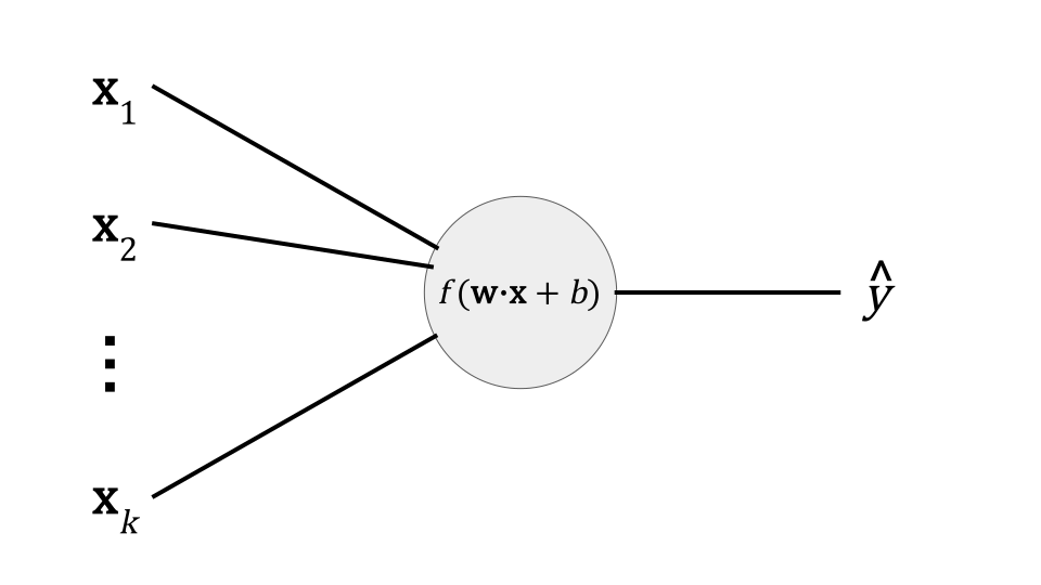
In last week's online lesson, we looked at models for classification that are more advanced than Naive Bayes. Specifically, we looked at models that are built on the idea of a generic "linear unit", which has the following mathematical form:
$$ \hat{y} = f(\mathbf{w} \cdot \mathbf{x} + b) $$
The key concepts here are:
- \( \mathbf{x} \) is a vector containing the input features.
- \( \mathbf{w} \) is a weight vector.
- \( b \) is a scalar bias term
- \( f \) is an activation function that maps the raw weighted sum to some finite output range (e.g., 0 to 1).
We call this "linear" because it matches the general mathematical formulation of a linear equation.
We also introducted the following simple visual representation of a single "linear unit":
Linear Classifiers
Next, we discussed how in practice, we want more than one output when doing classification tasks. Given a set of \( n \) possible classes \( C = \lbrace c_1,c_2,\dots,c_n \rbrace \), we want to represent how likely each class is for a given input \( \mathbf{x} \), which means we need \( n \) outputs. We can do this by having \( n \) copies of the "linear unit", as illustrated below:
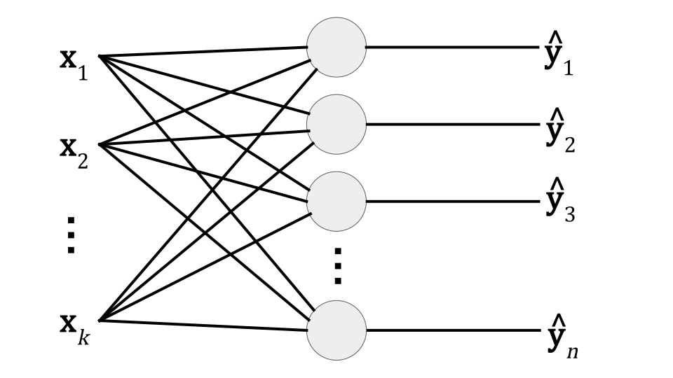
While you could implement this just by having a list of weights and biases and applying them in a loop, we discussed how this is mathmatically equivalent to doing a matrix multiplication and addition. We can define \( \mathbf{W} \) as a weight matrix where each row is the weight vector for one of the "linear units", \( \mathbf{b} \) as a bias vector containing the bias terms for each "linear unit", and \( F \) as some vector-level activation function. Then the equation for our multi-ouput classifier ends up becoming:
$$ \hat{\mathbf{y}} = F(\mathbf{W}\mathbf{x} + \mathbf{b}) $$
We concluded our discussion of linear classifiers by observing that the choice of activation function, loss function (i.e., measure of classifier error), and training algorithm effectively defines different types of linear classifiers. A threshold activation function (1 if the sum is above a threshold, 0 otherwise) results in a classifier known as a perceptron. The sigmoid activation function, combined with the logistic loss function and gradient descent training, results in a the logistic regression classifier.

There is also a distinct perceptron training algorithm, which we did not (and won't) cover.
Neural Networks
Finally, we discussed what happens if we want our classifier to use "fancier" features; that is, ones that can't be computed as simple functions on text. Examples might include conceptual questions like "is the text asking you to do something?" as a meaningful feature in spam detection.
Intuitively, we could imagine training a separate classifier to compute such "fancy features". The output of this classifier would then become the features that are sent as input to our final classifier. In other words, we wanted something like the following:
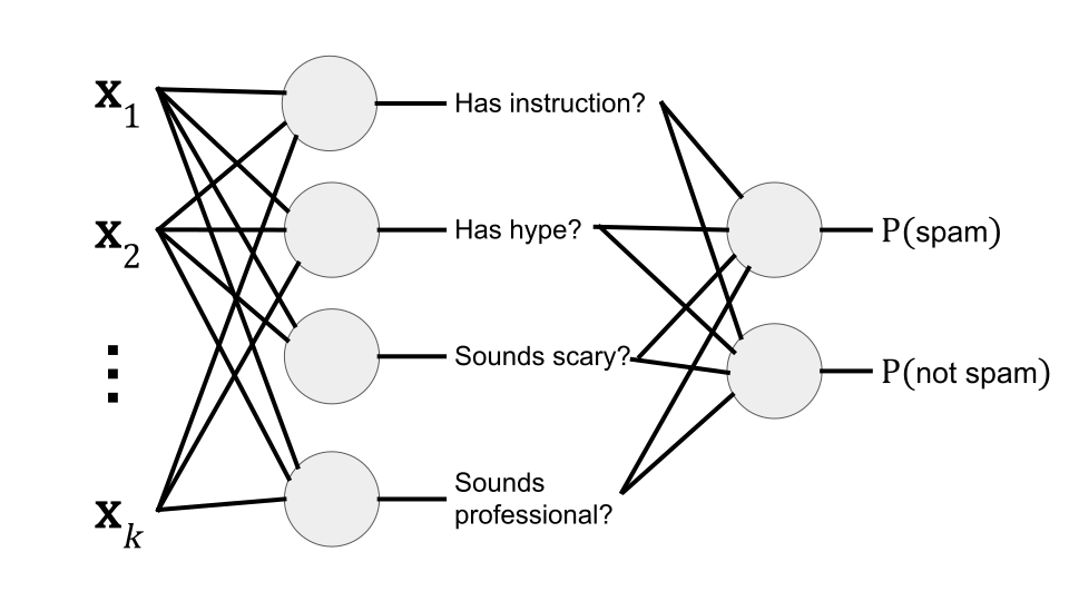
This type of classifier, consisting of multiple layers of "linear units", is known as a neural network.
And that's where we left off at the end of the lesson! We stopped just before getting to talk about how this idea might work in practice. That's our goal for this lesson!

And now, the conclusion!
(When logged in, completion status appears here.)