Geometrization of Bias

2021

Overview

The inductive orientation vector has been used to define algorithmic bias, entropic expressivity, algorithmic capacity, and more. This vector tells us how an algorithm distributes probability mass over a set of possible solutions. We develop a method to empirically estimate the inductive orientation vector for classification algorithms, unlocking an entire toolbox to help us understand the algorithms we use. We will clarify the meaning of the inductive orientation vector, describe how we find it, and apply it to compare algorithms.

The Meaning of Inductive Orientation

The inductive orientation vector encodes training data and an algorithm's inductive bias, making this vector specific to a given data-generating distribution and algorithm. An algorithm's inductive bias encompasses the assumptions built into a model, whether implicitly or explicitly. For example, a logistic regression classifier assumes that the data can be separated by a linear decision boundary, and many neural networks have a loss function that penalizes complex solutions, resulting in a bias for simpler solutions. However, many other inductive biases are more difficult to pinpoint and thus go unexplained. Our research provides a way to compare and contrast inductive biases, making algorithms' behavior more transparent and explainable. Since the inductive orientation vector depends only on data and the algorithm's inductive bias, any differences between algorithms trained on the same dataset must be due to differences in their inductive biases.

The Calculation of the Inductive Orientation Vector

To find the inductive orientation vector for an algorithm, we generate a Labeling Distribution Matrix (LDM) and take the average of its columns. The LDM was previously introduced by Sandoval Segura et al. Each column of the matrix describes the algorithm's expected probability distribution on all the possible labelings of a chosen holdout set when trained on a particular subset of the dataset. This means that between columns, we fix the algorithm and holdout set and vary the subset of the dataset used for training. Taking the average of the columns of the LDM generates the inductive orientation vector. We call each column of the LDM \(\overline{\mathbf{P}}_{F}\), where \(F\) represents the subset of data used for training, and we call the inductive orientation vector \(\overline{\mathbf{P}}_{\mathcal{D}}\), where \(\mathcal{D}\) is the data-generating process encapsulating the selection process of \(F\) from the overall dataset.

Select Applications and Results

Having generated our inductive orientation vectors, we explore their applications.

Inductive Orientation Vectors - Clustering - Benchmark Data Suite

Figure 1: Inductive Orientation Vectors calculated using the EEG Eye State Data Set from the UCI Machine Learning Repository.

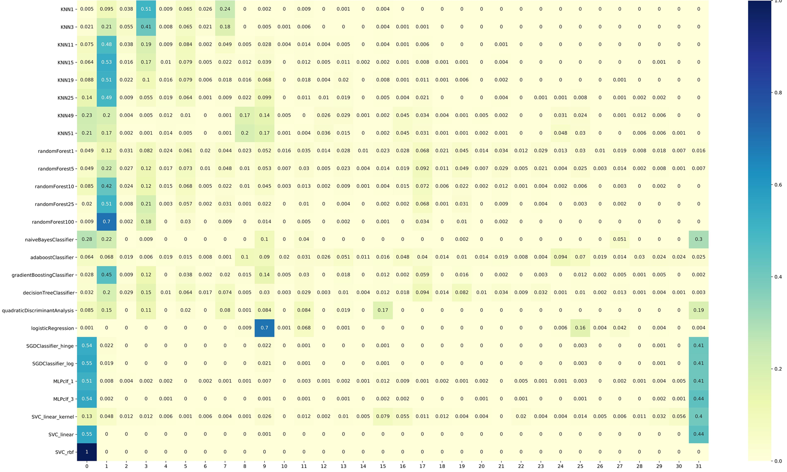
Each row in the above image represents an inductive orientation vector of the algorithms listed to the left. The 32 values of each vector represent the probability distribution over all possible ways of labeling a holdout set of 5 test instances, where each index corresponds to one sequence of labels. From this raw view of the inductive orientation vectors, we see some distinguishing features between the algorithms. For instance, classifiers that use stochastic gradient descent (SGD) as their optimizing method, Support Vector Classifiers (SVC), and Multilayer Perceptrons (MLP) seem to favor the 0th index. On the other hand, most Random Forest and K-Nearest-Neighbor (KNN) classifiers prefer the 1st index. We also see that different parameterizations of the same algorithms seem to have similar inductive orientations. Since we often assume that instances of the same algorithm with different parameters are generally similar, the fact that our estimated inductive orientation vectors can reflect these intrinsic similarities testifies to the potential of these vectors as a useful comparison tool.

Figure 2: The inductive orientation vectors, reduced to two dimensions using PCA, are plotted above. They are clustered at original dimensions using Meanshift and labeled accordingly. Note that the horizontal and vertical axes are generated in the dimensional reduction process and are essentially meaningless.

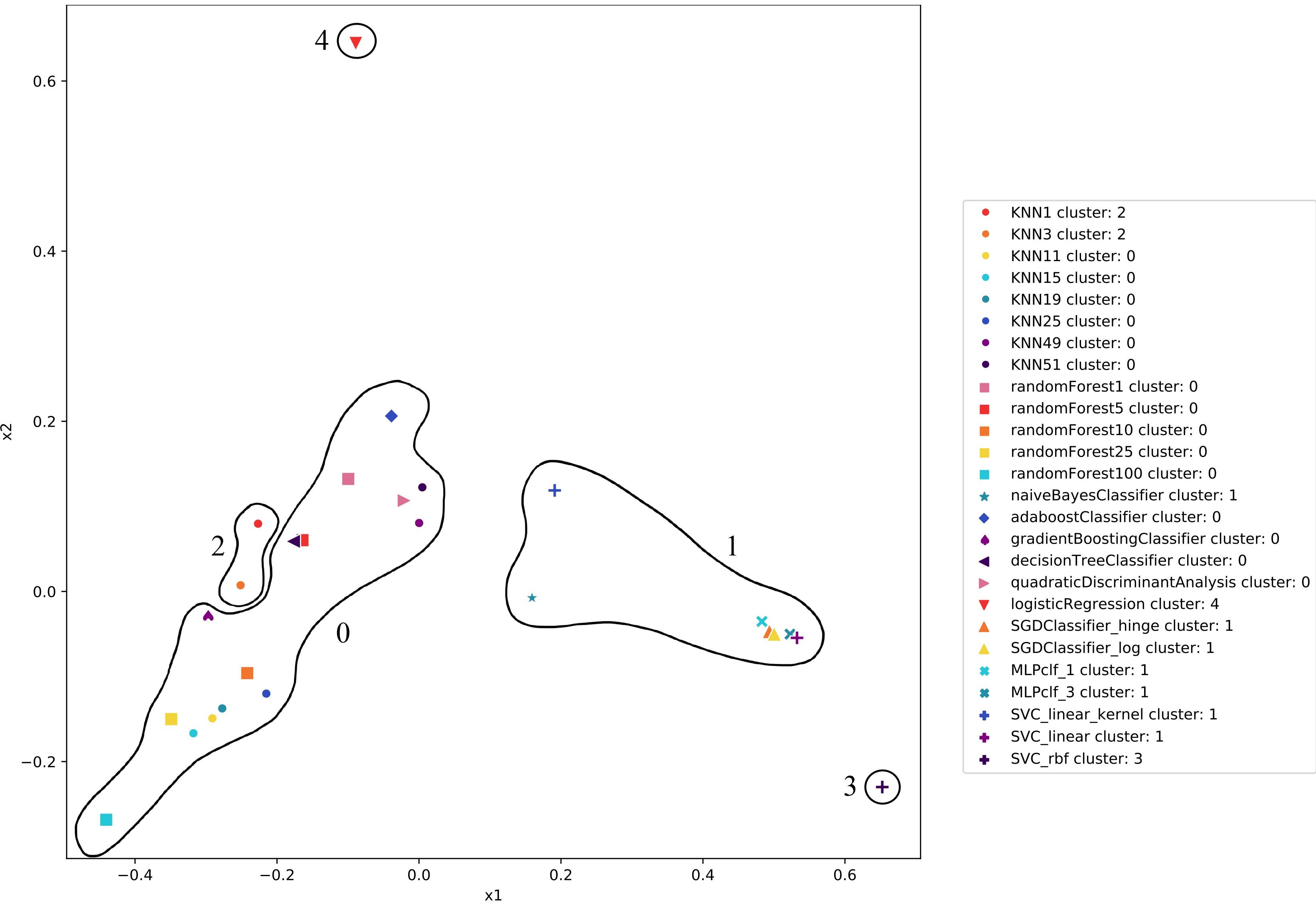
Aside from viewing the inductive orientation vectors as a probability distribution, we can take advantage of their geometric nature and visualize them in two dimensions. We observe that the relationships in our clustering plot are consistent with those that we saw in the inductive orientation vectors. For example, while most KNNs are close together, KNN1 and KNN3 have inductive orientation vectors that significantly differ from the rest and thus are clustered separately. Additionally, Random Forests are close to KNNs, and SVCs are close to MLPs, as expected. Thus, plotting inductive orientation vectors provides a powerful visual to qualify relationships between algorithms.

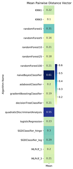
In our earlier results, we were only using the EEG Eye State dataset, and thus our analyses regarding the similarities in inductive orientations were limited. To make stronger statements regarding the algorithms' inductive biases, we need to see that whether their relationships remain consistent across datasets. To accomplish this, we use a matrix representing the pairwise distances between the inductive orientation vectors of algorithms across a set of benchmark datasets. We call this pairwise distance matrix the Benchmark Data Suite (BDS).

Figure 3: Each grid of the Benchmark Data Suite (top left) contains the distance between the inductive orientation vector of KNN11 and the algorithm designated by the row, trained on the dataset designated by the column. This distance is normalized by dividing by the maximum pairwise distance found in that column so that all our datasets are scaled the same way. The specific scaling factor for each dataset is represented by the Normalizing Constant Vector (bottom center). The average of the columns of the Benchmark Data Suite is presented as the Mean Pairwise Distance Vector (top right).

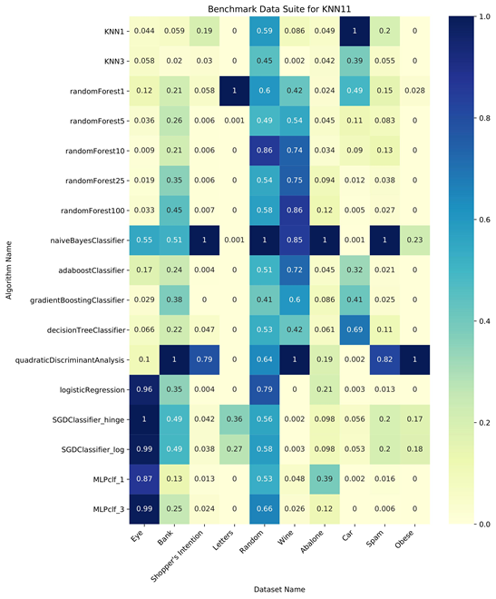
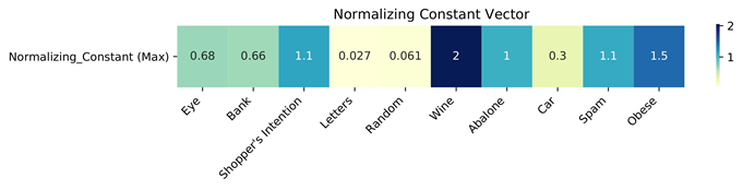
We observed that for the EEG Eye State dataset, KNN and Random Forest algorithms are closely related. Viewing the Benchmark Data Suite for KNN11, we see that this observation is valid for all datasets in the benchmark except the randomly generated dataset and the Wine Quality dataset. Existing research supports this relationship, as Lin and Jeon classify both algorithms as variants of weighted neighborhood schemes. Therefore, our inductive orientation vectors and analytical tools are valuable methods to uncover novel relationships between algorithms.

Algorithmic Bias, Entropic Expressivity, and Algorithmic Capacity

Finally, we turn to some applications of the inductive orientation vector developed in past AMISTAD research - algorithmic bias, entropic expressivity, and algorithmic capacity. We will provide a short description of each, followed by more detailed formal definitions, before diving into some results. For a more complete discussion of these topics, please refer to their respective papers.

• Algorithmic Bias - Algorithmic bias measures how much better (or worse) a learning algorithm performs in comparison to randomly guessing solutions. This bias differs from inductive bias because algorithmic bias considers how well the algorithm predicts solutions while inductive bias only considers what kind of predictions the algorithm prefers.
• Entropic Expressivity - Entropic expressivity captures the spread of an algorithm's probability distribution using the Shannon entropy of the inductive orientation vector. In other words, the more evenly the probability mass is distributed, the higher the entropic expressivity, with a uniform probability distribution having maximum entropic expressivity.
• Algorithmic Capacity - Algorithmic capacity measures the flexibility of an algorithm's probability distribution as the training data changes. Intuitively, an algorithm that adapts and conforms according to its training data has a higher algorithmic capacity than an algorithm that is fixed.

Algorithmic Bias

In statistics, the bias of a process is defined as expected deviation from a ground truth quantity, such as how much more likely an event will be compared to random chance. We follow this notion of deviation from a random ground-truth for defining algorithmic bias. In our case, the process is the algorithm, the event is classifying a holdout set of test features at or above the desired accuracy, and the random chance is represented by randomly guessing the labels of the holdout set. Formally, we can write this in terms of the inductive orientation vector as $$\text{Bias}(\mathcal{D},\mathbf{t}) = \mathbf{t}^{\top}\overline{\mathbf{P}}_\mathcal{D} - \frac{\|\mathbf{t}\|^2}{|\Omega|},$$ where \(\mathcal{D}\) is a distribution over a space of information resources, \(\mathbf{t}\) is a fixed k-hot target function, \(|\Omega|\) is the size of the search space (the number of possible classifications) and \(\overline{\mathbf{P}}_\mathcal{D}\) is the inductive orientation vector. In other words, algorithmic bias is the difference between an algorithm's probability of success and the probability of success when choosing uniformly at random.

Entropic Expressivity

Another use of the inductive orientation vector is determining the entropic expressivity of an algorithm. The entropic expressivity measures the ability of an algorithm to distribute its probability mass over the search space in expectation. Mathematically, $$\text{Entropic Expressivity} = \mathit{H}(\overline{\mathbf{P}}_\mathcal{D}) = \mathit{H}(\mathcal{U})-\mathit{D}_{\mathbf{KL}}(\overline{{\mathbf{P}}}_{\mathcal{D}}||\mathcal{U}),$$ where \(\mathit{D}_{\mathbf{KL}}(\overline{\mathbf{P}}_{\mathcal{D}}||\mathcal{U})\) is the Kullback-Leibler divergence between the inductive orientation vector \(\overline{{\mathbf{P}}}_{\mathit{D}}\) and the uniform distribution \({\mathcal{U}}\) over the search space \({\Omega}\), and \(H(\cdot)\) denotes the Shannon entropy.

Entropic expressivity measures the uniformity of an algorithm's preference over solutions in the search space. An inductive orientation vector with higher entropic expressivity has a more uniform probability distribution. A length 4 inductive orientation vector with maximum entropic expressivity would have the form [0.25 0.25 0.25 0.25]. Algorithms with high entropic expressivity do not favor any particular solution, thus they are less biased.

Algorithmic Capacity

The algorithmic capacity for an algorithm \(\mathcal{A}\) and a fixed data distribution \(\mathcal{D}\) can be written in terms of the entropic expressivity, namely, $$\text{Algorithmic Capacity} = C_{\mathcal{A}, \mathcal{D}} = H(\overline{\mathbf{P}}_\mathcal{D})-\mathbb{E}_\mathcal{D}[H(\overline{\mathbf{P}}_{F})].$$ Imagine a fairly uniform \(\overline{\mathbf{P}}_\mathcal{D}\) vector. It could be uniform because all the \(\overline{\mathbf{P}}_{F}\) vectors are uniform, or because they are all sparse in different directions. Algorithmic capacity allows us to distinguish between these two causes, as we subtract the expectation of the entropic expressivity of the \(\overline{\mathbf{P}}_{F}\) vectors from the entropic expressivity of the inductive orientation \(\overline{\mathbf{P}}_\mathcal{D}\).

• If the \(\overline{\mathbf{P}}_{F}\) vectors are uniform, their entropic expressivity will be high, causing the algorithmic capacity of the algorithm to be low. Such an algorithm does not respond to changes in data.
• Conversely, if the \(\overline{\mathbf{P}}_{F}\) vectors are sparse in different directions, their entropic expressivity would be low, causing the algorithmic capacity to be comparatively higher. Such an algorithm does respond to changes in data.

Thus, algorithmic capacity measures how much an algorithm restructures its probability distribution when trained on different information resources. The greater this value is, the greater the ability to adapt and store information.

Results

Algorithm	Entropic Expressivity	Algorithmic Capacity	Algorithmic Bias
KNN1	2.109	2.109	0.700
KNN3	2.377	2.377	0.685
KNN11	2.477	2.477	0.585
KNN49	3.257	3.257	0.023
KNN51	3.176	3.176	-0.009
Random Forest1	4.661	1.134	0.165
Random Forest5	4.089	1.099	0.301
Random Forest10	3.120	0.421	0.440
Random Forest25	2.424	0.833	0.610
Random Forest100	1.512	0.813	0.719
Naive Bayes	2.335	2.335	0.081
Adaboost	4.521	4.517	-0.052
Gradient Boosting Classifier	2.860	2.811	0.458
Decision Tree	3.960	3.244	0.376
Quadratic Discriminate Analysis	3.087	3.087	0.240
Logistic Regression	1.474	1.474	-0.120
SGD Classifier (Hinge Loss)	1.308	0.150	-0.164
SGD Classifier (Log Loss)	1.288	0.147	-0.168
MLP Classifier (1 layer)	1.661	0.338	-0.169
MLP Classifier (3 layer)	1.778	0.138	-0.184
SVC_linear_kernel	3.313	3.313	-0.095
SVC_linear	1.020	0.055	-0.187
SVC_rbf	0.000	0.000	-0.188

Table 1: Entropic expressivity, algorithmic capacity, and algorithmic bias calculated using the inductive orientation vectors generated on the EEG Eye State Dataset. Algorithmic bias is computed for a target set that accepts predictions with at least 4 out of 5 labels correct.

Our results show that many KNNs and Random Forests have high bias while SVCs and MLPs struggled, performing even worse than random guessing as shown by their negative bias. We also saw evidence for the bias-expressivity trade-off previously explored by our lab: as the algorithmic bias of random forests parameterizations increased, entropic expressivity decreased. Note that the bias-expressivity trade-off describes the boundary relationships between those two properties, so it is still possible for some algorithms to not follow the trend.

Authors

Acknowledgments

We would like to thank all the AMISTAD members who helped expand the Algorithmic Search Framework and the theory around inductive orientation vectors. This research was supported in part by the National Science Foundation under Grant No. 1950885. Any opinions, findings or conclusions expressed are the authors' alone, and do not necessarily reflect the views of the National Science Foundation.

Further Reading

• Bashir, D., Montañez, G. D., Sehra, S., Sandoval Segura, P., and Lauw, J. (2020). An Information-Theoretic Perspective on Overfitting and Underfitting. Australasian Joint Conference on Artificial Intelligence (AJCAI 2020)
• Lauw, J., Macias, D., Trikha, A., Vendemiatti, J., and Montanez, G. D. (2019). The bias-expressivity-trade-off.arXiv preprint arXiv:1911.04964.
• Montañez, G.D., Hayase, J., Lauw, J., Macias, D., Trikha, A., Vendemiatti, J. :The Futility of Bias-Free Learning and Search. 2nd Australasian Joint Conference on Artificial Intelligence (AI 2019), 2019. 277—288
• Montañez, G.D. The Famine of Forte: Few Search Problems Greatly Favor Your Algorithm. In: 2017 IEEE International Conference on Systems, Man, and Cybernetics(SMC). pp. 477—482.