Lab 2: Frequency and N-Grams

In lecture, we talked about how even though word frequencies seem like a simple and crude tool, they can actually be super useful for discovering cool things about language! One early interesting discovery relating to word frequencies is known as Zipf's Law. First put to writing in 1932 by linguist George Zipf (hence the name), Zipf's law states, in plain English, that the frequency of a word is inversely proportional to its rank in a frequency-ordered list. Or, mathematically:

$$ C(w) \propto \frac{1}{K(w)} $$, or equivalently, $$ C(w) = \frac{S}{K(w)} $$

Where \( w \) is a token, \( C(w) \) is the frequency (count) of \( w \) (as defined in class), \( K(w) \) is its rank in a frequency-ordered list (so the highest frequency word has rank \( K(w)=1 \), the second highest \( K(w)=2 \), etc.), and \( S \) is an arbitrary constant (which you can think of as a scaling factor).

If you're curious to learn more, check out Wikipedia's page on Zipf's Law.

In this part of the lab, we'll put Zipf's Law to the test! We will use matplotlib to visualize the relationship between frequency and rank. Matplotlib is a plotting library for Python with syntax inspired by MATLAB, and is very commonly used in science writing—so if you've never used it before, this is your chance to learn and practice a very useful tool!

Part 1a: read_one and read_all

Instead of writing our own tokenization functions, we will use spaCy to do the tokenization. Pause now and read a bit about spaCy language processing pipelines.

For this part, we only want spaCy to tokenize our text, so we will set the pipeline to have no steps using the empty list, []. Since some of our documents will be long, but we’re not doing any memory-intensive processing, we will tell spaCy that it’s okay to load large documents all at once instead of a little bit at a time. To specify these instructions, add these lines to the top of your zipf.py file:

from spacy.lang.en import English

nlp = English(pipeline=[], max_length=5000000)

Next, write a function called read_one(file_path) that takes the location of a file as its input, and that returns a Counter object representing all of the tokens in the corresponding text file. (Please lowercase all of the text!)

Hint: You can get the Token objects in a spaCy document by iterating over a spaCy Doc object, e.g. using Python's for...in loop syntax. You can get the text of a Token (as a string) using the .text attribute of the Token object.

Hint: The following is a standard Pythonic way to open a latin1-encoded file with name filename as read-only ('r'). This is a nice alternative to having to call both open and close on a file.

with open(filename, 'r', encoding='latin1') as fp: 
    # do processing...

Next, write a function called read_all(dir_path, extension=None) that takes the location of a directory as its input, and returns a Counter object representing all of the text of all of the (lowercased) files in the corresponding directory whose file extention is extension. If extension is None, then read_all should include every file in the directory. For example, read_all("/courses/cs159/data/gutenberg", ".txt") should return a Counter that counts all of the tokens in all of the text files saved with the .txt extension in the /courses/cs159/data/gutenberg directory, while ignoring all other files (e.g., .md files) in that directory.

Hints: You will want to use the os.walk function to recursively search for files in the directory. You can get a file’s extension with os.path.splitext. It may also be helpful to know that two Counter objects can be added together to create a new Counter object!

Part 1b: do_zipf_plot

Although Zipf's Law was originally defined in terms of absolute frequency (count), in NLP it's often more common to reason in terms of relative frequencies, \( R(w) \) as defined in class. (you can take a moment to convince yourself that, assuming a fixed corpus, this shouldn't affect the proportionality relationship at all!) The reason we prefer relative frequency is that the scale of absolute counts depends on the corpus size (bigger corpus means bigger numbers), whereas relative frequency is always between 0 and 1, making it easier to compare across corpora.

Let \( R(w) \) be the relative frequency of \( w \) as defined in class (e.g. if "the" occurs 1642 times out of 35652 tokens, then its relative frequency is 1642/35652 = 0.04606), and \( K(w) \) be the rank as defined above. To visualize the relationship between rank and frequency, we will create a log-log plot of \( K(w) \) (on the x-axis) versus \( R(w) \) (on the y-axis). For these plots, we will use the pyplot library, part of matplotlib.

By default, matplotlib will try to open a window to display figures as soon as they’re created. That won’t work over ssh (unless you’re using window forwarding) or in VS Code, but we can stop matplotlib from trying to open the plot in a new window by changing which backend it uses; that is, what it does with information about a plot once it's rendered. This needs to be done before we import pyplot using the following incantation:

import matplotlib
matplotlib.use('Agg')
from matplotlib import pyplot

You will write a function called do_zipf_plot that takes two parameters: - A Counter object with the counts of words from one or more files. - A string label that can be used to title the figure.

The starter code includes two implemented functions that call do_zipf_plot: - plot_one, which calls read_one and do_zipf_plot to generate a visualization of data from one file, and - plot_all, which calls read_all and do_zipf_plot to generate a visualization of data from an entire directory.

Your do_zipf_plot function should start by creating a figure object:

fig = pyplot.figure()

It should then use the Counter argument to create data in the right form for a call to pyplot.loglog.

Be sure to label your axes and plot with xlabel, ylabel, and suptitle functions in pyplot. Add a legend to the lower left of the plot (you can explore the pyplot documentation for how to do this), and then save the resulting figure:

pyplot.savefig('zipf_{}.png'.format(label))
pyplot.close()

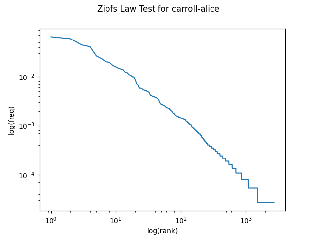
Before moving on, confirm that calling plot_one('/courses/cs159/data/gutenberg/carroll-alice.txt') generates a plot that matches the one below:

Part 1c: Testing Zipf's Law

Now we're ready to test how well Zipf's Law works! Per the equations above, the 50th most common word should occur with about three times the frequency of the 150th most common word (for example).

Add to your do_zipf_plot function so that in addition to plotting the empirical rank vs frequency data, it also plots the expected values using Zipf’s law. For the constant scaling factor \( S \) in the formulation of Zipf's Law above, you should use:

$$ S = \frac{T}{H(n)} $$

So that the computation for expected frequency works out to be:

$$ C(w) = \frac{S}{K(w)} = \frac{T}{H(n)K(w)} $$

where \( T \) is the number of word tokens in the corpus, \( n \) is the number of word types in the corpus, and \( H(n) \) is the \( n \)th harmonic number. (Remember: the number of tokens is the total number of words in the document. The number of types is the total number of unique words in the corpus.)

Use this function to compute harmonic numbers. It’s included in your starter code:

def H_approx(n):
    """
    Returns an approximate value of n-th harmonic number.
    http://en.wikipedia.org/wiki/Harmonic_number
    """
    # Euler-Mascheroni constant
    gamma = 0.57721566490153286060651209008240243104215933593992
    return gamma + math.log(n) + 0.5/n - 1./(12*n**2) + 1./(120*n**4)

To plot a second curve, you will add a second pyplot.loglog(...) line after you plot the empirical frequency data. Be sure to label each data line so that your legend will be informative!

WARNING: Be careful about the scales of your y-axis when plotting the two curves! Notice that the math gives you expected absolute frequencies \( C(w) \), but the curve we plotted in Part 1b was scaled to relative frequencies \( R(w) \). Some additional scaling will probably be needed, otherwise your two curves will look way different by orders of magnitude!

Analysis Question #1

Zipf’s Law and Alice: How closely does the empirical data in carroll-alice.txt follow the theoretical relationship of Zipf's Law?

Analysis Question #2

Zipf’s Law and Other Texts: Repeat the previous question for a few other texts of your choice included in the /courses/cs159/data/gutenberg directory. Are the results consistent? In your answer, please be sure to name the specific texts you chose and the plots for each of them.

Analysis Question #3

Zipf’s Law and All Texts: Repeat the Zipf’s Law experiment with all of the text from all of the files in /courses/cs159/data/gutenberg. How many tokens are in this combined corpus? How does this plot compare with the plots from the smaller corpora? Once again, please make sure to include the resulting plot in your answer.

Analysis Question #4

Zipf’s Law Discussion: Does Zipf’s Law hold for each of the plots your made? What intuitions have you formed? Does the length of a document have an impact on how well it does or does not follow Zipf’s Law? What else do you notice?

Analysis Question #5

Zipf’s Law for Random Text: Generate synthetic (that is, "fake") random text by using random.choice("abcdefg... "), taking care to include the space character in your text. You will need to import random first. Use the string join command to accumulate your random characters into a (very) long string. Then tokenize this string, and generate the Zipf plot as before, and compare the plot to the ones you got from your non-synthetic English data. What do you make of Zipf’s Law in the light of this? (Source: Exercise 23b, Bird, Klein and Loper, 2009) Once again, please make sure to include the resulting plot in your answer.

(When logged in, completion status appears here.)