Module 08.1: Lambda Calculus — Computation with Nothing but Functions

In earlier modules, we learned to write programs using functions, to represent programs as data, and to give those programs meaning by evaluating them.

Now we're going to examine a very small language that gets rid of almost everything we normally expect from a programming language.

No numbers. No Booleans. No lists. No built-in conditionals. No named function definitions. No loops.

There are just variables, function definitions, and function applications.

This language is called the untyped lambda calculus (λ-calculus). Despite its simplicity, it is powerful enough to express general computation. We'll learn its rules in this module, then use them to construct familiar programming concepts in Modules 08.2 and 08.3.

By the end of this module, you should be able to read and write lambda expressions; identify a function's parameter, body, bound variables, and free variables; perform simple β-reductions; explain why α-renaming matters; distinguish reduction from normal form; and use the lc interpreter on the CS 131 server to experiment.

How to use this module

When you see a box labeled Gradescope question, answer that question in the Module 8.1 Completion assignment on Gradescope.

Near the end, you'll run a few experiments with lc on the CS 131 server and describe what you saw.

---

Why Invent a Language This Small?

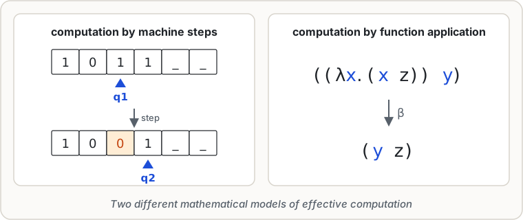
In the 1930s, mathematicians were trying to make the informal idea of effective computation precise. What, exactly, does it mean for something to be computable by following a mechanical procedure?

Alan Turing approached this question with machines that manipulate symbols according to explicit rules. Alonzo Church approached it using functions and symbolic substitution. His system became the lambda calculus.

These approaches look very different. One emphasizes changes to the state of a machine; the other emphasizes function application. Yet they characterize the same broad class of computable functions. This is one reason both are central to the foundations of computer science.

Lambda calculus also connects directly to our course:

• In Haskell, we've treated functions as values that can be passed around, returned, and applied.
• When building interpreters, we've used substitution, environments, and scope to explain what programs mean.
• When studying abstraction, we've asked how much machinery is really necessary to express an idea.

Lambda calculus takes that last question to an extreme: how much computation can we express if functions are almost all we have?

---

The Entire Language

Here is the grammar of our small language:

expr ::= variable
       | (expr expr)
       | (λ variable . expr)

For now, assume variables are single lowercase letters such as x, y, and z. We will write expressions with all their parentheses so the structure is completely clear.

There are only three kinds of expressions.

A variable

x

This is a complete, valid lambda expression. So are y and z.

A variable is just a symbol. Unlike a number, it doesn't inherently represent a particular value. Its meaning depends on whether some enclosing lambda abstraction binds it.

A function application

(f x)

This means: apply f to x.

The left expression is the function; the right expression is the argument.

Importantly, both parts can be arbitrary lambda expressions, not just letters:

((λx.x) y)

The function is (λx.x) and the argument is y.

A lambda abstraction

(λx.x)

This represents an anonymous function: a function with parameter x and body x.

Its Haskell equivalent is:

\x -> x

Another example:

(λx.y)

This is a function that ignores its parameter x and has the body y.

Note that lambda calculus has no built-in Haskell values or operations. For now, expressions such as x + 1, True, or [1,2] are not pure lambda-calculus expressions. We'll learn how to represent things like these using functions.

The whole language at a glance

In this table, M and N stand for any lambda expressions.

Form	Shape	Example	Haskell analogue
Variable	x	y	y
Application	(M N)	((λx.x) y)	(\x -> x) y
Abstraction	(λx.M)	(λx.y)	\x -> y

That's everything. Every lambda expression you'll ever see is built by nesting these three forms.

Parentheses are structure

In our fully parenthesized notation, every application has exactly two parts, a function and one argument. So the placement of parentheses determines what gets applied to what, and two expressions with the same letters can mean very different things:

Expression	Means
((f x) y)	apply f to x, then apply the result to y
(f (x y))	apply x to y first, then pass that result to f

You may encounter the convenient abbreviation f x y, which usually means ((f x) y). Similarly, some writing omits outer parentheses or writes λx.λy.x instead of (λx.(λy.x)). These abbreviations are helpful once the underlying structure is clear. While learning the rules, we'll always write every parenthesis.

Gradescope question: Recognizing lambda expressions

Submit this response on Gradescope.

Using the fully parenthesized grammar above, select all the syntactically valid lambda expressions:

• x
• (λx.x)
• (x y)
• ((λx.x) z)
• (x y z)
• (λx.(y x))
• (λx.3)
• ((x y) z)

Choose one invalid expression and explain briefly which part of the grammar it violates.

---

Functions, Parameters, and Scope

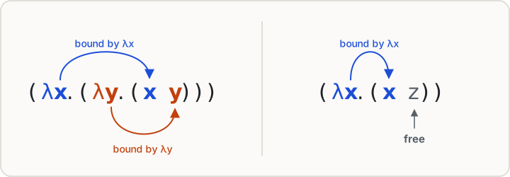
Every lambda abstraction has two parts: a parameter (the variable right after λ) and a body (everything after the dot). Here are the parts of (λx.(x y)):

The λx binds the occurrences of x in its body. y has no λy around it, so nothing binds it.

This should sound familiar: we discussed scope when building interpreters with environments and closures.

Definition: bound and free occurrences

An occurrence of a variable is bound if it sits inside the body of a lambda with that same parameter name. The nearest such lambda is its binder. An occurrence that no lambda binds is free.

"Bound" and "free" describe occurrences, not names. The same letter can be bound in one place and free in another.

Bound variables

In:

(λx.(x x))

both occurrences of x in the body are bound by the λx at the beginning. The body can use its parameter more than once, just as a Haskell function can.

Free variables

In the diagram above, y is free: there is no enclosing λy to bind it.

A free variable is not necessarily an error. We can work with open expressions, whose meaning depends on something outside the expression, just as a Haskell function body can mention a name defined elsewhere in the file.

Nested scopes

Consider:

(λx.(λy.(x y)))

The inner body (x y) uses both parameters:

• x is bound by the outer lambda.
• y is bound by the inner lambda.

Now consider:

(λx.(λx.x))

Here the occurrence of x in the innermost body is bound by the inner λx, the nearest one. The inner binder shadows the outer one, just as an inner let or lambda parameter shadows an outer variable of the same name in Haskell.

The picture below summarizes both ideas: each bound occurrence points back to its binder, and anything with no binder is free.

Gradescope question: Bound and free

Submit this response on Gradescope.

Consider:

(λx.(λy.(x z)))

Which variable occurrences are bound, and which are free? Identify the binder for each bound occurrence.

---

Computation by β-Reduction

In an ordinary programming language, applying a function means supplying an argument and evaluating the function body.

Lambda calculus formalizes that basic idea with β-reduction (pronounced "beta reduction").

Start with the identity function:

(λx.x)

Apply it to y:

((λx.x) y)

To evaluate the application:

1. Find the parameter (x).
2. Find the function body (x).
3. Replace the occurrences of x in the body that this λx binds with the argument (y).

The result is:

((λx.x) y)  →β  y

Read M →β N as "M reduces to N in one β-step." This is one β-reduction step.

Definition: β-reduction

An application whose function part is a lambda abstraction, ((λx.body) arg), takes one β-step to a copy of body in which every occurrence of x bound by that λx is replaced by arg. The λx and the argument disappear.

A more interesting body

Consider:

((λx.(x z)) y)

We substitute y for x in the body (x z):

(x z)       -- original body
(y z)       -- after substitution

Therefore:

((λx.(x z)) y)  →β  (y z)

Notice that we do not replace z. Only the occurrences bound by the parameter being applied are replaced.

A function that ignores its argument

((λx.z) y)  →β  z

The body contains no occurrence of the parameter x, so substitution changes nothing: the argument is simply thrown away.

Functions returning functions

Consider:

((λx.(λy.x)) a)

The outer function takes an argument and returns another function:

((λx.(λy.x)) a)  →β  (λy.a)

The resulting function remembers a in its body and ignores whatever argument is later passed for y.

This is the lambda-calculus version of a familiar Haskell idea: currying and partial application.

For example, the Haskell function:

\x -> \y -> x

returns a function after receiving its first argument.

A two-step computation

Now apply two arguments. The innermost application, ((λx.(λy.x)) a), is reduced first, and its result is then applied to b:

   (((λx.(λy.x)) a) b)
→β ((λy.a) b)              -- substitute a for x
→β a                       -- substitute b for y (y does not appear)

One argument at a time, exactly as with curried Haskell functions.

β-reduction versus evaluating arithmetic

Our reduction steps manipulate expressions, not machine integers. The symbols a, b, and z are variables, not secretly numbers. Lambda calculus will only acquire something like numeric computation once we build an encoding for numbers.

Gradescope question: Perform a reduction

Submit this response on Gradescope.

Show the β-reduction steps for:

(((λx.(λy.(y x))) a) b)

What is the resulting expression? Briefly identify what gets substituted in each step.

---

α-Equivalence: Names Aren't the Important Part

These are the same function, except that we chose different names for its parameter:

(λx.x)
(λw.w)

We say that they are α-equivalent ("alpha equivalent"). In Haskell, it's the same idea as these two definitions being interchangeable:

\x -> x
\w -> w

Definition: α-equivalence

Two expressions are α-equivalent if one can be turned into the other by renaming bound variables, where each renaming changes a binder and exactly the occurrences it binds, and never changes which binder any occurrence belongs to. Free variables are never renamed.

For instance, compare some candidates against (λx.(x z)):

Expression	α-equivalent to (λx.(x z))?	Why
(λw.(w z))	yes	renamed the binder x and its one occurrence to w
(λw.(w w))	no	the free z became bound by λw
(λx.(x y))	no	changed a free variable, z to y

Why renaming can matter during substitution

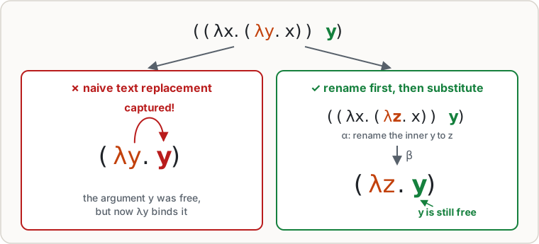
Suppose we try to reduce:

((λx.(λy.x)) y)

A naive text replacement would turn the body (λy.x) into (λy.y), the identity function. That's wrong! Before substitution, the argument y is a free variable. In the naive result, it has become bound by λy. This is called variable capture.

To avoid it, first rename the inner bound variable y to a fresh name, say z. That gives an α-equivalent expression (written =α), which we can then safely reduce:

   ((λx.(λy.x)) y)
=α ((λx.(λz.x)) y)         -- rename the inner y to z
→β (λz.y)                  -- substitute y for x

Here the y remains free, exactly as it should.

When you try this in lc later in this module, you'll see it do the same renaming automatically: it picks the fresh name y' and prints (λy'.y).

This is capture-avoiding substitution: when reducing an application, we preserve which variable occurrences are free and which are bound.

---

Reduction Order, Normal Forms, and Nontermination

A lambda expression can sometimes contain more than one place where β-reduction is possible.

Definition: redex and normal form

A redex (short for reducible expression) is any subexpression of the form ((λx.body) argument): a lambda abstraction applied to an argument, ready for a β-step.

An expression is in normal form when it contains no redexes, so no β-step is possible.

For example, y is in normal form, and so is (λx.x): neither contains a lambda abstraction applied to an argument. (y z) is also in normal form. It is an application, but its function part y is a variable, not a lambda, so there is nothing to substitute into.

Some computations never finish

Consider:

Ω = ((λx.(x x)) (λx.(x x)))

The name Ω is just a convenient abbreviation.

What happens if we reduce it?

The function body is (x x). Substitute the argument (λx.(x x)) for both occurrences of x:

   ((λx.(x x)) (λx.(x x)))
→β ((λx.(x x)) (λx.(x x)))   -- the same expression again
→β ...

We are back where we started, so the same step can repeat forever. Not every lambda expression has a normal form.

Does reduction order matter?

Consider:

((λx.z) Ω)

The outer function ignores its argument. If we reduce that outer application first, we get z immediately.

If we insist on reducing Ω first, we can get stuck reducing forever.

This echoes something we learned about lazy evaluation in Haskell: evaluating an unused argument may be unnecessary, and in some cases doing so would prevent termination.

We won't develop a complete theory of reduction strategies here. The important ideas are that a β-reduction is a precise local rule, and that different choices about what to reduce next can affect whether we reach a result.

Gradescope question: Normal form and nontermination

Submit this response on Gradescope.

Why can:

((λx.z) Ω)

reduce to z even though Ω never reaches a normal form?

(Here Ω abbreviates ((λx.(x x)) (λx.(x x))).)

---

Try Lambda Calculus on the CS 131 Server

You've learned the reduction rules by hand. Now you can use a small interpreter to see them in action.

The CS 131 server has an interpreter called lc.

Open a terminal on the server (cs131.cs.hmc.edu) the same way you do for labs and homework, and run:

lc

(See Connecting to the Server with VS Code if you haven't gotten to a terminal on the server yet.)

You should see an lc> prompt. This is an interactive interpreter, much like GHCi, but for lambda calculus rather than Haskell.

Typing a lambda

You can't easily type λ, so the interpreter accepts a backslash in its place: typing (\x.x) means (λx.x), just like Haskell's \x -> x. When lc prints expressions back to you, it uses the real λ.

When you enter an application, lc shows each β-reduction step it takes, followed by the final result and a count of total steps. For example, entering ((\x.(x x)) w) prints the following (on the server, the redex is also underlined and colored):

lc> ((\x.(x x)) w)

After 0 β-reductions:

    ((λx.(x x)) w)
  →ᵦ
    (w w)

(w w)

1 total steps

Each "After n β-reductions" block shows one step: the expression before it, the arrow, and the expression after it. The line on its own near the end is the final result.

Try these expressions in order. Make a prediction before pressing Enter, and pay attention to how many β-reduction steps you see.

Experiment A: the identity function

((\x.x) y)

Predict: what should the result be? How many β-reduction steps should lc display?

Experiment B: substitution into an application

((\x.(x z)) y)

Predict which occurrence changes and which one stays unchanged.

Experiment C: a function that returns a function

((\x.(\y.x)) a)

The result should itself be a lambda abstraction. What does that returned function do?

Experiment D: two applications

(((\x.(\y.(y x))) a) b)

Try to anticipate the intermediate expression after the first reduction.

Experiment E: make your own

Invent a short application using an anonymous function, perhaps one that ignores its argument or uses its argument twice. Evaluate it with lc.

Useful interpreter commands

Enter :help to see the available commands. For example, :set trace compact shortens the reduction output, :set trace full brings back every step, and :load filename.lc loads definitions from a file. In Lab 08, you'll load a provided .lc file. For this module, you only need the interactive prompt.

If your results look different from your handwritten work, first check the parentheses and then compare which redex the interpreter reduces at each step. Different valid reduction sequences may reach α-equivalent results.

Gradescope question: Your lc experiments

Submit this response on Gradescope.

What result did you get for Experiment B, and how many β-reduction steps did the interpreter display?

Then describe Experiment E: show the expression you tried and say what happened. Did the result match your prediction? If not, what did you learn?

---

What to Carry Forward

The lambda calculus is built entirely from three forms: variables, applications, and abstractions.

The key operation is β-reduction: apply a function by substituting an argument for its parameter in the body, while respecting scope.

Three ideas make that rule precise:

• Free and bound occurrences: the same name can refer to different things in different scopes.
• α-equivalence: bound-variable names can change without changing the meaning.
• Capture avoidance: substitution must not accidentally change which variables are bound.

Some expressions reduce to normal forms; others reduce forever.

In the next module, we'll confront an apparent problem: if our entire language consists of functions, where do Booleans, numbers, pairs, and lists come from?

Rather than adding new primitive constructs, we'll encode them as functions.

---

Finish Module 08.1

Check that you submitted the five Gradescope questions encountered above:

1. Recognizing syntactically valid expressions
2. Bound and free variables
3. A β-reduction
4. Normal form and nontermination
5. Your lc experiments

Gradescope question: Time spent

Submit this response on Gradescope.

Approximately how much time did you spend on this module?

• less than 30 minutes
• 30 - 45 minutes
• 45 - 60 minutes
• 60 - 75 minutes
• 75 - 90 minutes
• more than 90 minutes

Gradescope question: Lingering questions

Submit this response on Gradescope.

What lingering questions or thoughts do you have about this module?